Art with Neural Network

風格, 創作這種能力在現在Alpha Go已經稱霸的時代, 目前覺得還是人類獨有的
不過有趣的是, 對於那些已經在 ImageNet 訓練得非常好的模型, 如: VGG-19, 我們通常已經同意模型可以辨別一些較抽象的概念
那麼是否模型裡, 也有具備類似風格和創作的元素呢? 又或者風格在模型裡該怎麼表達?
本篇文章主要是介紹這篇 A Neural Algorithm of Artistic Style 的概念和實作, 另外一個很好的投影片 by Mark Chang 也很值得參考
先給出範例結果, 結果 = 原始的內容 + 希望的風格
- Content Image

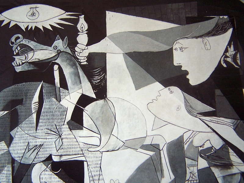
- Style Image
- Result Image

說在前頭的最佳化
在講下去之前, 我們先講 NN 的事情, 一般情況, 我們是給定 input image x, 而參數 w 則是要求的變數, 同時對 loss (objective function) 做 optimize, 實作上就是 backprob.
上面講到的三種東西列出來:
- x: input image (given, constant)
- w: NN parameters (variables)
- loss: objective function which is correlated to some desired measure
事實上, backprob 的計算 x and w 角色可以互換. 也就是將 w 固定為 constant, 而 x 變成 variables, 如此一來, 我們一樣可以用 backprob 去計算出最佳的 image x.
因此, 如果我們能將 loss 定義得與風格和內容高度相關, 那麼求得的最佳 image x 就會有原始的內容和希望的風格了!
那麼再來就很明確了, 我們要定義出什麼是 Content Loss 和 Style Loss 了
Content Loss
針對一個已經訓練好的 model, 我們常常將它拿來做 feature extraction. 例如一個 DNN 把它最後一層辨識的 softmax 層拿掉, 而它的前一層的 response (做forward的結果), 就會是對於原始 input 的一種 encoding. 理論上也會有很好的鑑別力 (因最只差最後一層的softmax).
Udacity 的 traffic-sign detection 也有拿 VGG-19, ResNet, 和 gooLeNet 做 feature extraction, 然後只訓練重新加上的 softmax layer 來得到很高的辨識率.
因此, 我們可以將 forward 的 response image 當作是一種 measure content 的指標!
知道這個理由後, 原文公式就很好理解, 引用如下:
So let p and x be the original image and the image that is generated and Pl and Fl their respective feature representation in layer l. We then define the squared-error loss between the two feature representations
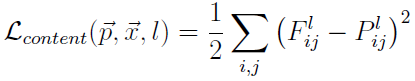
簡單來說 Pl 是 content image P 在 l 層的 response, 而 Fl 是 input image x (記得嗎? 它是變數喔) 在 l 層的 response.
這兩個 responses 的 squared-error 定義為 content loss, 要愈小愈好. 由於 response 為 input 的某種 encoded feature, 所以它們如果愈接近, input 就會愈接近了 (content就愈接近).
引用 Mark Chang 的投影片: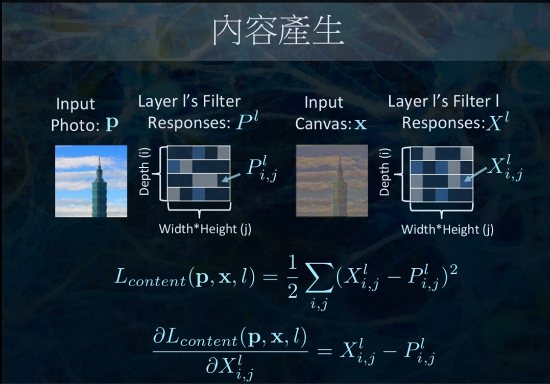
Style Loss
個人覺得最神奇的地方就在這裡了! 當時自己怎麼猜測都沒猜到可以這麼 formulate.
我個人的理解是基於 CNN 來解釋
假設對於某一層 ConvNet 的 kernel 為 w*h*k (width, hieght, depth), ConvNet 的 k 通常代表了有幾種 feature maps
說白一點, 有 k 種 filter responses 的結果, 例如第一種是線條類的response, 第二種是弧形類的responses … 等等
而風格就是這些 responses 的 correlation matrix! (實際上用 Gram matrix, 但意義類似)
基於我們對於 CNN 的理解, 愈後面的 layers 能處理愈抽象的概念, 因此愈後面的 Gram matrix 也就愈能代表抽象的 style 概念.
原文公式引用如下:
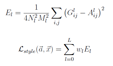
總之就是計算在 l 層上, sytle image a 和 input image x 它們的 Gram matrix 的 L2-norm 值
一樣再一次引用 Mark Chang 的投影片: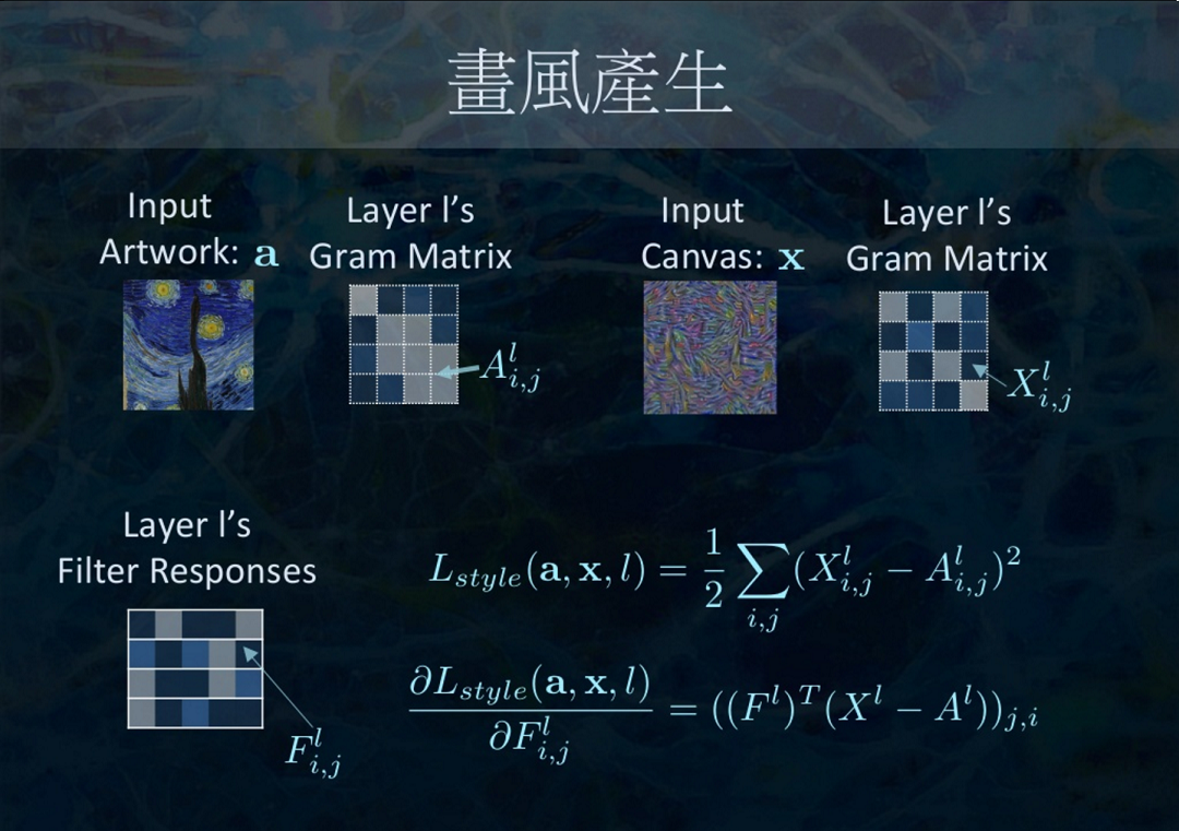
也可以去看看他的投影片, 有不同角度的解釋
實戰
主要參考此 gitHub
一開始 load VGG-19 model 就不說了, 主要的兩個 loss, codes 如下:
|
|
一開始給定 random input image: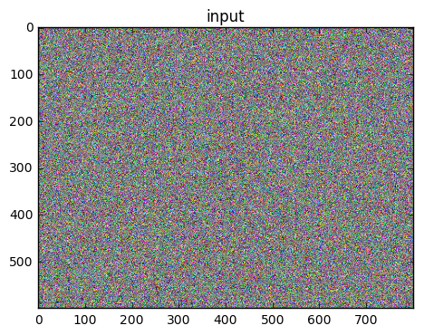
style image 選定如下: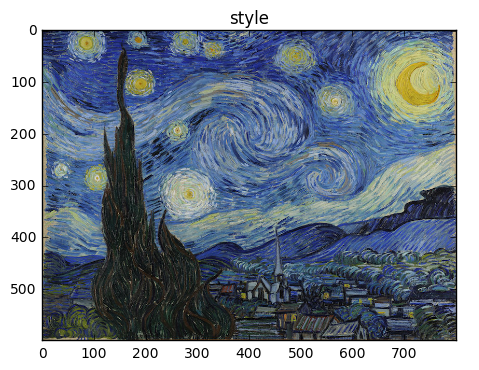
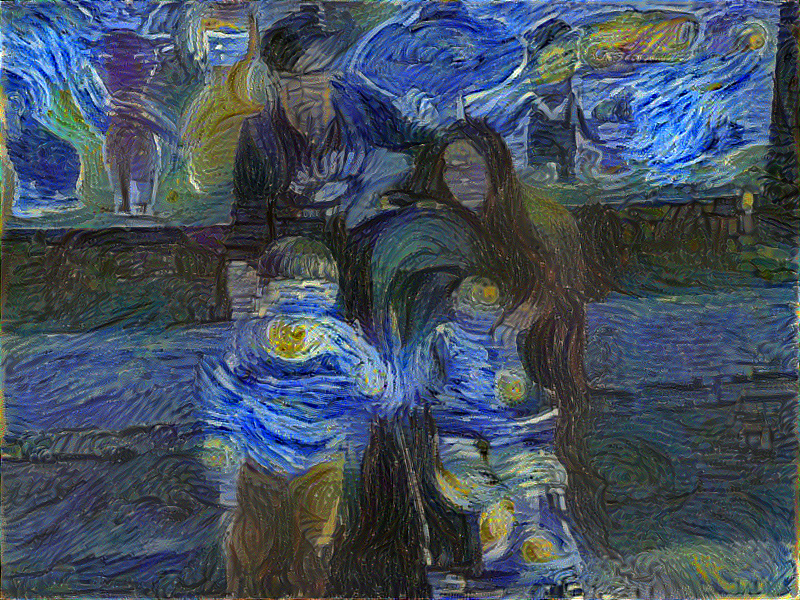
隨著 iteration 增加會像這樣:
- 第一次的 backprob:

- 1000 iteration:

- 2000 iteration:

- 3000 iteration:
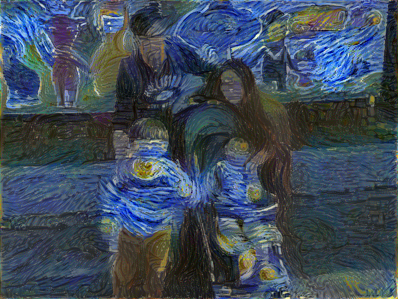
- 4000 iteration:
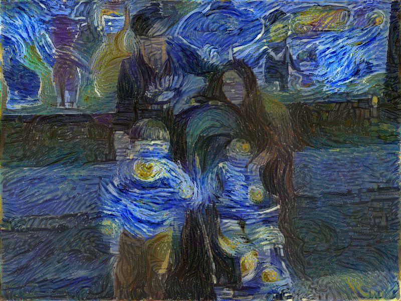
- 5000 iteration:
短節
這之間很多參數可以調整去玩, 有興趣可以自己下載 gitHub 去測
上一篇的 “GTX 1070 參見” 有提到, 原來用 CPU 去計算, 1000 iteration 花了六個小時! 但是強大的 GTX 1070 只需要 6 分鐘!
不過, 就算是給手機用上GTX1070好了 (哈哈當然不可能), 6分鐘的一個結果也是無法接受!
PRISMA 可以在一分鐘內處理完! 這必定不是這種要算 optimization 的方法可以達到的.
事實上, 李飛飛的團隊發表了一篇論文 “Perceptual Losses for Real-Time Style Transfer and Super-Resolution“
訓練過後, 只需要做 forward propagation 即可! Standford University 的 JC Johnson 的 gitHub 有完整的 source code!
找時間再來寫這篇心得文囉!