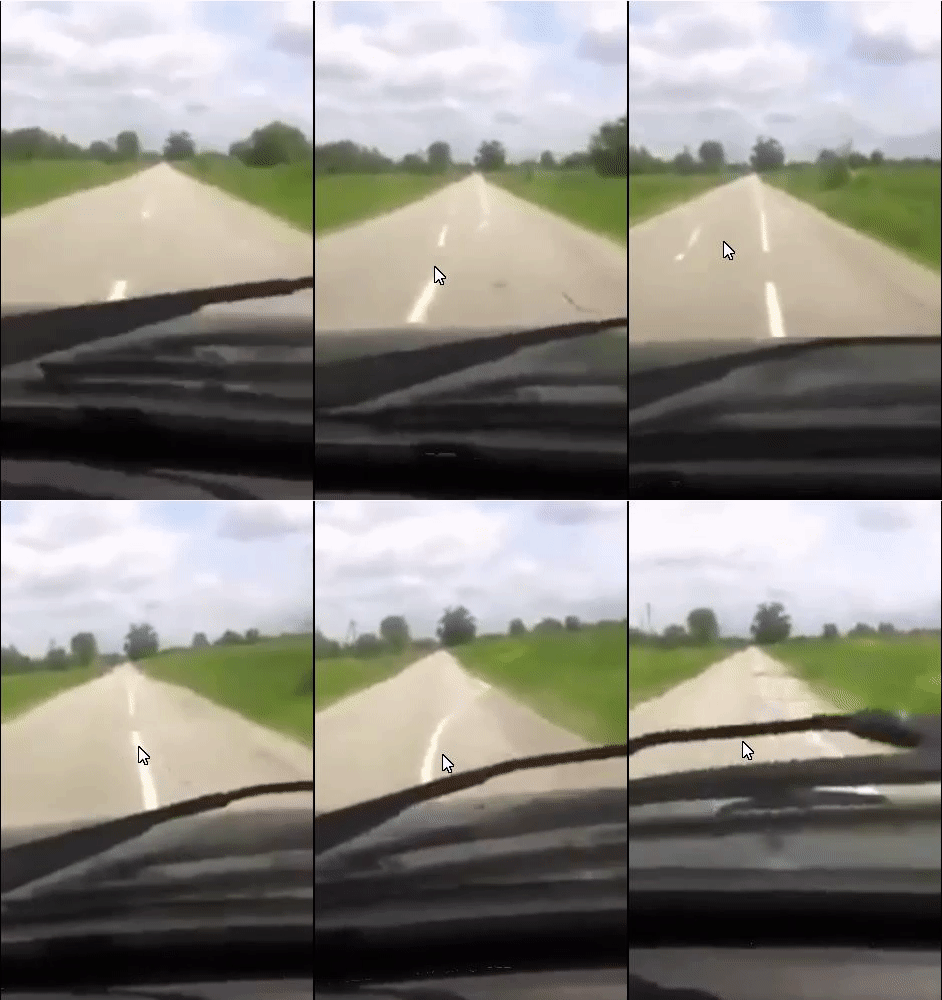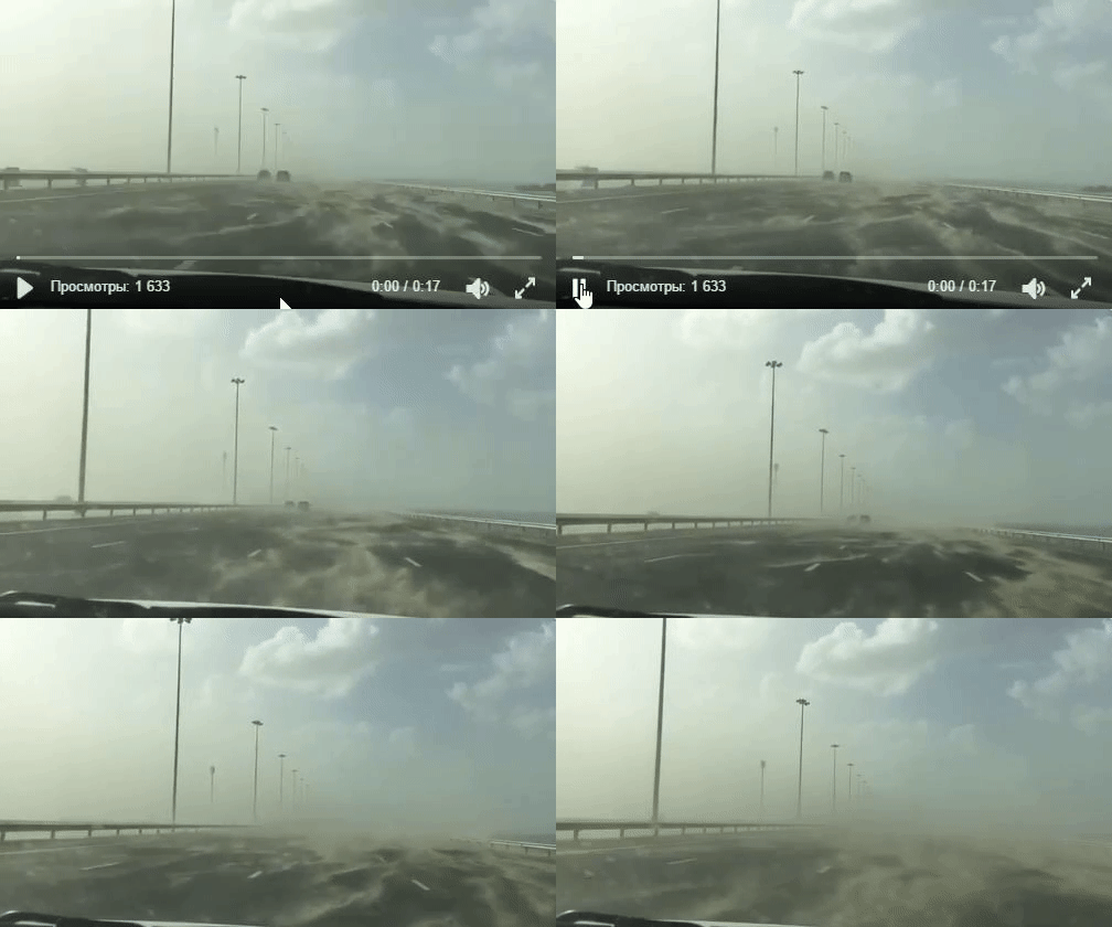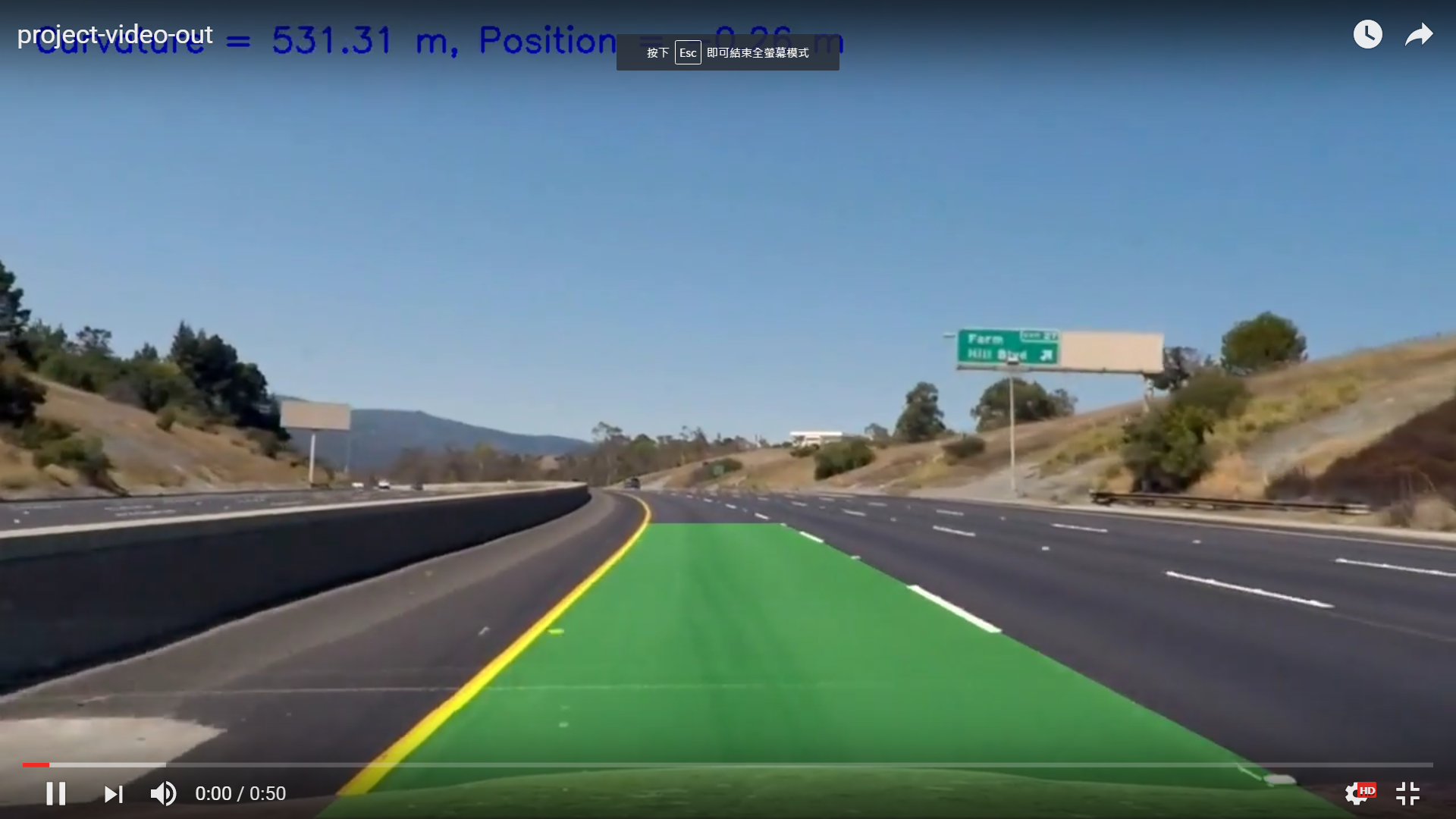
以下是 github 上的 README, 全英文. 此 Project 主要都是在做 Computer Vision 相關的東西. 學到了許多使用 Python and CV 相關的技巧. 整理來說是個滿有趣的 project!
The goals / steps of this project are the following:
- Compute the camera calibration matrix and distortion coefficients given a set of chessboard images.
- Apply a distortion correction to raw images.
- Use color transforms, gradients, etc., to create a thresholded binary image.
- Apply a perspective transform to rectify binary image (“birds-eye view”).
- Detect lane pixels and fit to find the lane boundary.
- Determine the curvature of the lane and vehicle position with respect to center.
- Warp the detected lane boundaries back onto the original image.
- Output visual display of the lane boundaries and numerical estimation of lane curvature and vehicle position.
Rubric Points
1. Camera calibration
The images for calculating the distortion and 3-D to 2-D mapping matrix are stored in ./camera_cal/calibration*.jpg.
Firstly, I used cv2.findChessboardCorners to find out all those corner points (corners) in the images.
Then I used cv2.calibrateCamera to calculate the distortion (dist) and mapping matrix (mtx) given the corners pts and their corresponding predifined 3-D pts objp
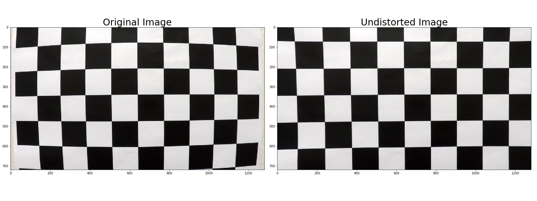
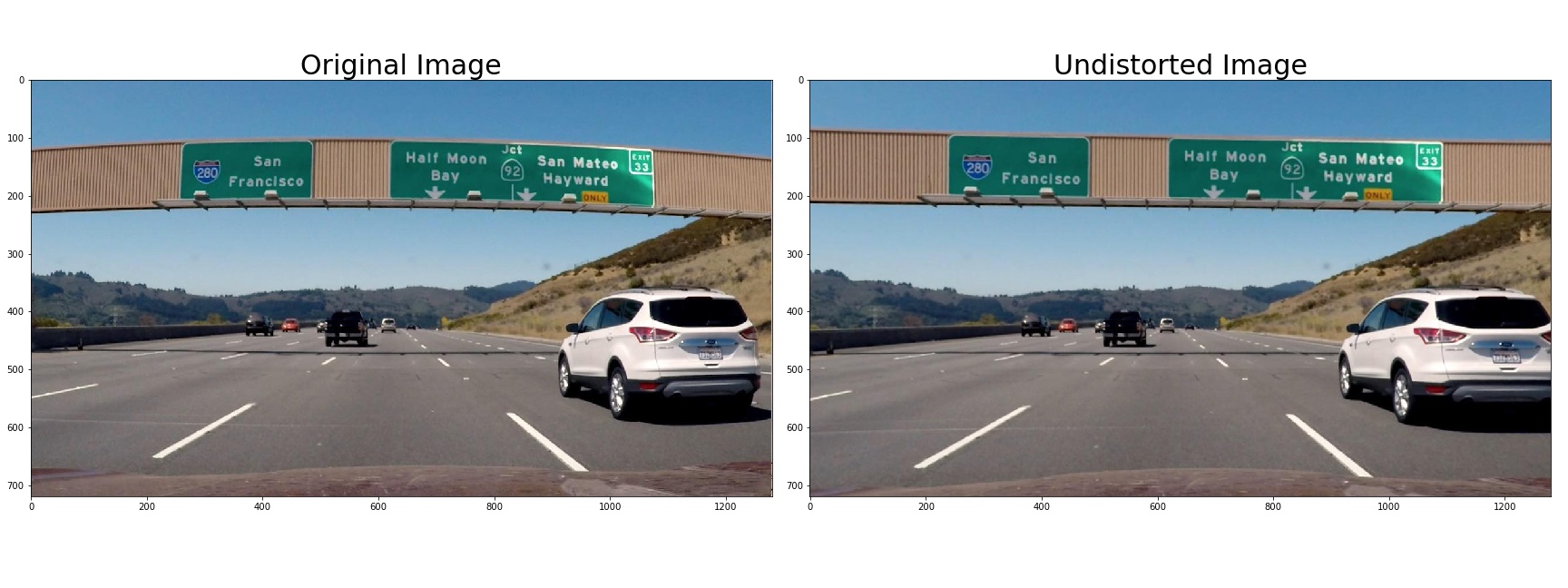
2. Provide an example of a distortion-corrected image
Here is an example of distortion-corrected image:
3. Create a thresholded binary image and provide example
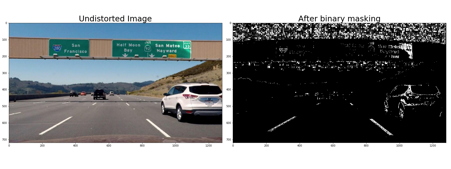
I used magnitude of gradients, direction of gradients, and L and S in HLS color space.
A combined rule is used:
|
|
Example masking image is showed:
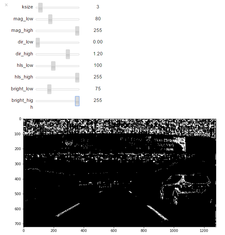
Moreover, I used widgets to help tunning the parameters of those masking functions. It can provide instantaneous binary result that really help for accelarating this step. The widgets codes are list here:
|
|
4. Perspective transform
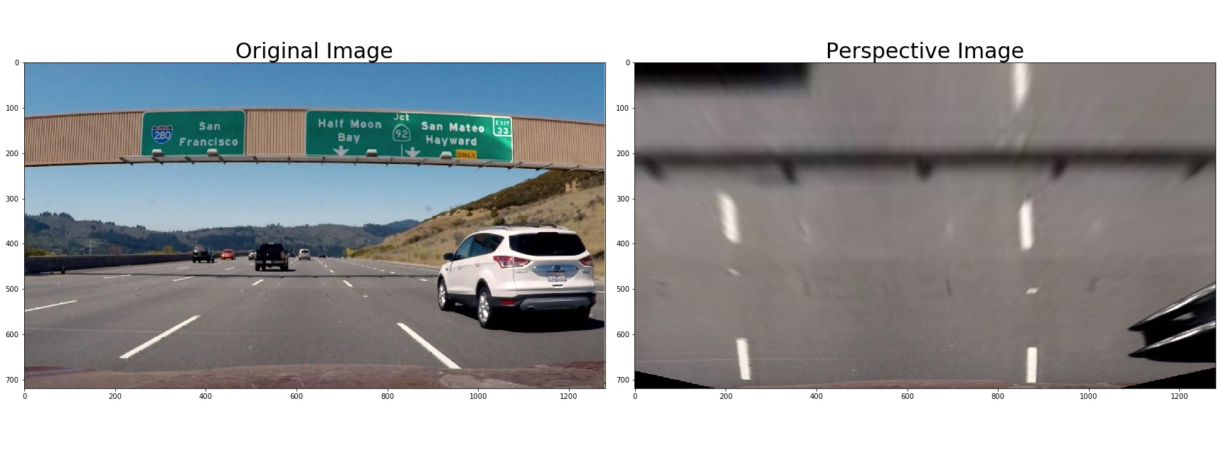
First, I defined the source and destination of perspective points as follows:
| Source | Destination |
|---|---|
| 585, 460 | 320, 0 |
| 203, 720 | 320, 720 |
| 1127, 720 | 960, 720 |
| 695, 460 | 960, 0 |
Then the perspective_warper function is defined which returns perspective image and the matrix warpM as well.warM is needed for the later step which does the inverse perspective back to the original image.
|
|
An example is showed here:
5. Lane line pixel and polynomial fitting
I applied a windowing approach to identify the lane pixels
![]()
In this example, I used 9 windows for both lane lines. The window is processed in an order from the buttom to the top.
Pixels are detected by the following function
|
|
lcenter_inandrcenter_inare the centers (in horizontal coordinate) of windows.win_numdefines how many windows are used. In this example, 9.win_half_widthrefers to the half length of window widthstart_from_buttonindicates how the initial centers of windows are set. Specifically, Let the current window as j and current frame index as i. Ifstart_from_button=True, the center of window j will be initally set as window j-1. Otherwise, it will be initally set as window j in frame i-1. Then, by using the initial position just set, the lane pixels are identified if the histogram of that window is high enough. Finally, based on those identified pixels, update the center position of current widnow j.
Next, a simple second order polynomial fitting is applied to both identified pixels
|
|
![]()
But wait! Since we are assuming “birds-eye view”, both lanes should be parallel!
So I first tried a method that ties the polynomial coefficients except the shifting ones!
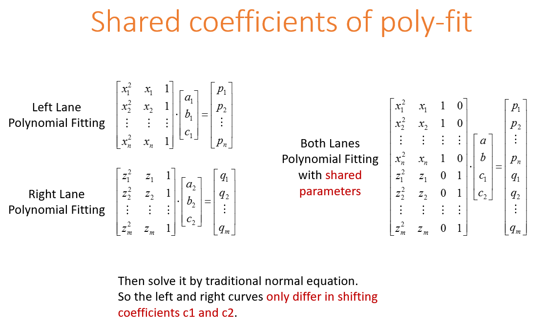
this method results in the following example
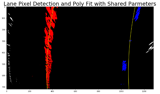
As can be seen in the figure, curves are indeed parallel. However, when I applied this method to the final video, I found that it wobbling a lot! (see “8. Video” below)
After some investigation, I wonder that this problem is caused by the fixed source points of perspective.
Since the pre-defined source points are always at the center of the camera while the lane curves are usually not, the result perspective curves is intrinsically not parellel!
Hence, I applied a dynamic source point correction. Idea of method is showed in the follows:
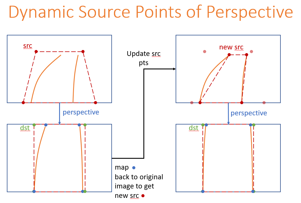
mapping inversely from coordinates in perspective images to original images can use the following formula:
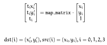
and results in the following example

It works great! Unfortunately, if the lane curves are not stable, the resulting new source points may fail. This is the major difficulty of this method! (see “8. Video” below)
6. Radius of curvature of the lane and the position of the vehicle
The curvature is calculated based on the following formula. Udacity provides a very good tutorial here !
|
|
There’s no need to worry about absolute accuracy in this case, but your results should be “order of magnitude” correct.
So I divide my result by 10 to make it seems more reasonable. And of course, the “order of magnitude” remains intact.
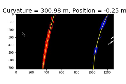
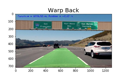
7. Warp the detected lane boundaries back onto the original image
In order to warp back onto the original image, we need to calculate the inverse of perspective transform matrix warpM
just apply Minv = inv(warpM) which is from numpy.linalg import inv
Then, simply apply cv2.warpPerspective with Minv as input.
Note: use cv2.putText to print the curvature and position onto images
8. Video

Simple poly-fit (Most stable! Simple is better ?!)
Shared coefficients of poly-fit (Wobbling problem)
Dynamic source points of perspective (Unstable, crash sometimes. If the lane curves are not stable, the resulting new source points may fail)
Discussion
Basically, I applied those techniques suggested by Udacity.
I did some efforts trying to parallize both curves in the perspective “bird eye view”. Two methods are applied
- Shared coefficients of polynomial fitting
- Dynamic source points of perspetive
Each has its own issue. For (1.), wobbling, and for (2.) unstable.
Future works will focus on solving the (2.) unstable issue. Maybe a smoothing method is a good idea.
Moreover, for more difficult videos, pixels may not be detected which makes the pipeline crash.
One way to overcome this problem is when this issue happens, the lane curve is set to be the same as previous frame.
Generelizing this idea, a confidence measure of lane pixels is worth to apply. If the confidence is low, then set the lane curve as the same as previous frame might be a good way to better estimate result.
Finally, finding a robust combination of masking rule and tweaking those parameters precisely might help too.
附上中文其他討論:
Reviewer 給了很多有用的 article links! 這邊附上做未來參考
- Perspective bird eye view:
http://www.ijser.org/researchpaper%5CA-Simple-Birds-Eye-View-Transformation-Technique.pdf
https://www.ncbi.nlm.nih.gov/pmc/articles/PMC3355419/
https://pdfs.semanticscholar.org/4964/9006f2d643c0fb613db4167f9e49462546dc.pdf
https://pdfs.semanticscholar.org/4074/183ce3b303ac4bb879af8d400a71e27e4f0b.pdf- Lane line pixel identification:
https://www.researchgate.net/publication/257291768_A_Much_Advanced_and_Efficient_Lane_Detection_Algorithm_for_Intelligent_Highway_Safety
https://www.ncbi.nlm.nih.gov/pmc/articles/PMC5017478/
https://chatbotslife.com/robust-lane-finding-using-advanced-computer-vision-techniques-46875bb3c8aa#.l2uxq26sn- lane detection with deep learning:
http://www.cv-foundation.org/openaccess/content_cvpr_2016_workshops/w3/papers/Gurghian_DeepLanes_End-To-End_Lane_CVPR_2016_paper.pdf
http://lmb.informatik.uni-freiburg.de/Publications/2016/OB16b/oliveira16iros.pdf
http://link.springer.com/chapter/10.1007/978-3-319-12637-1_57 (chapter in the book Neural Information Processing)
http://ocean.kisti.re.kr/downfile/volume/ieek1/OBDDBE/2016/v11n3/OBDDBE_2016_v11n3_163.pdf (in Korean, but some interesting insights can be found from illustrations)
https://github.com/kjw0612/awesome-deep-vision (can be useful in project 5 - vehicle detection)
噁心到吐血的真實挑戰:
還是老話一句, 真的要成為可用的產品, 難道超級無敵高阿!!
