TF Notes (3), Computational Graph in Tensorflow

這篇介紹 computational graph (計算圖譜), 主要來源參考自李宏毅教授的課程內容. 並且我們使用 tensorflow 的求導函數 tf.gradients 來驗證 computational graph. 最後我們在 MNIST 上驗證整個 DNN/CNN 的 backpropagation 可以利用 computational graph 的計算方式訓練.

Computational Graph

主要就截圖李教授的投影片, 一個 computational graph 的 node 和 edge 可以定義如下

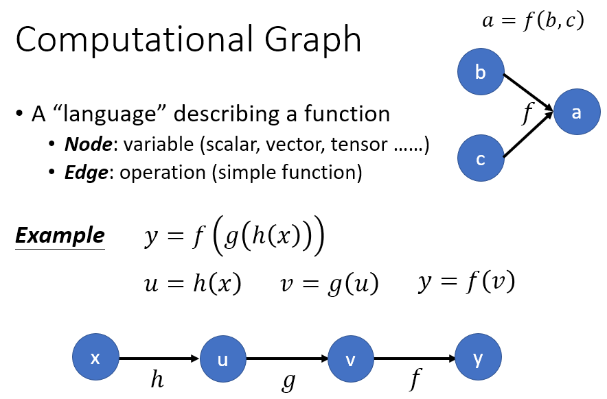
對於 chain rule 的話, 我們的計算圖譜可以這麼畫

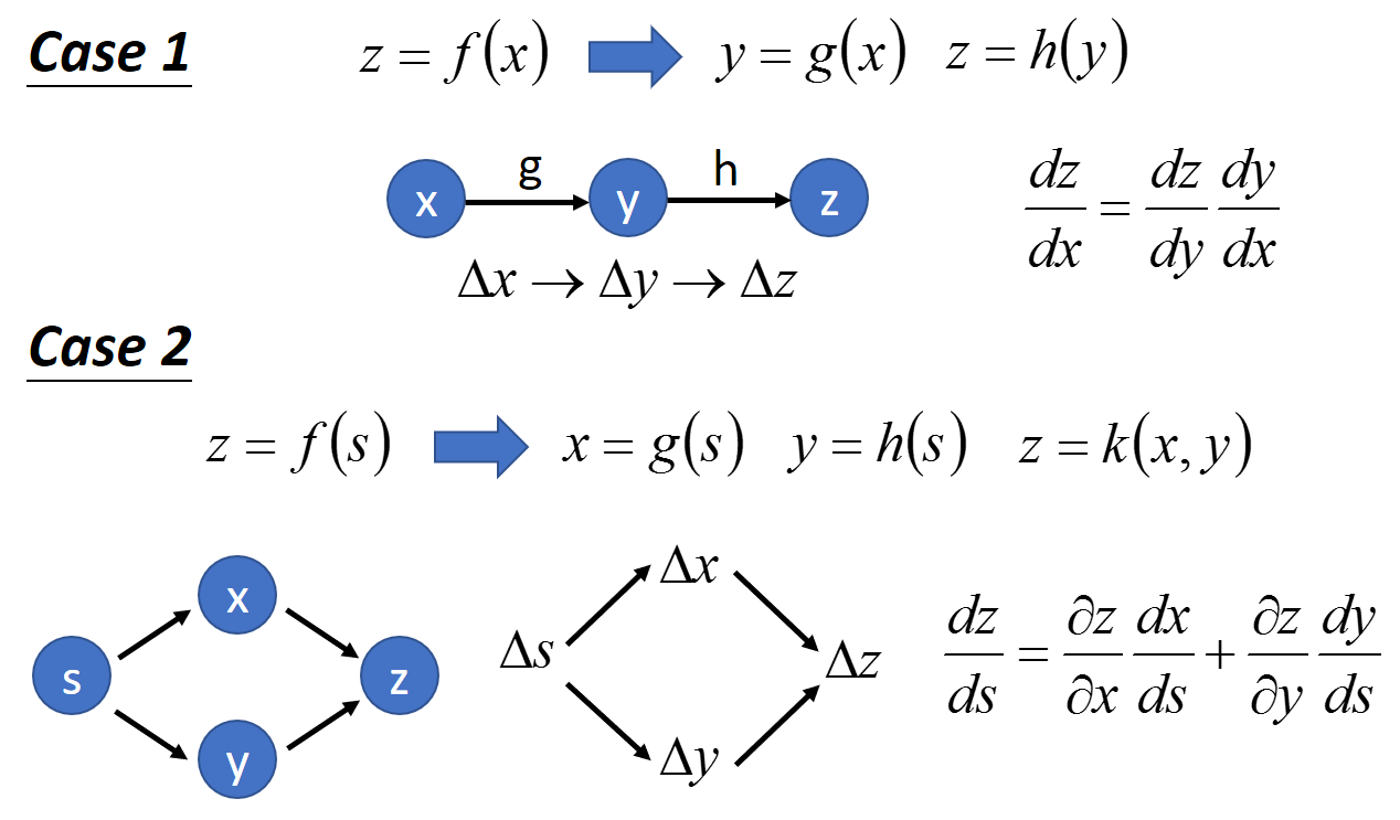
其實就是 chain rule 用這樣的圖形表示. 比較要注意的就是 case 2 的情況, 由於 $x$ and $y$ 都會被 $s$ 影響, 因此計算 gradients 時要累加兩條路徑.

再來另一項要注意的是如果有 share variables 我們的計算圖譜該怎麼表示呢 ? 舉例來說如下的函式
$y=x\cdot e^{x^2}$

計算圖譜畫出來長這樣

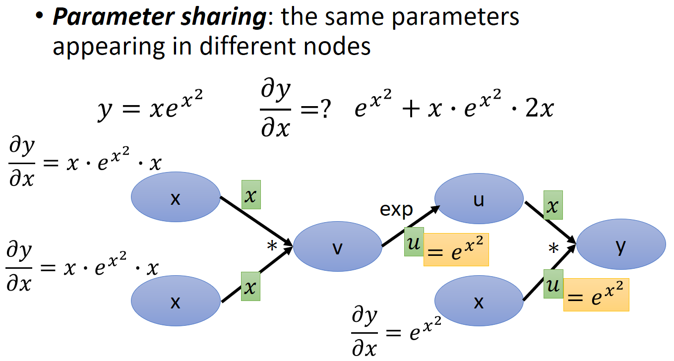
簡單來說把相同變數的 nodes 上所有的路徑都相加起來. 上面的範例就是計算 $\frac{\partial y}{\partial x}$ 時, 有三條路徑是從 node $x$ 出發最終會影響到 node $y$ 的, 讀者應該可以很容易看出來.

另外如果分別計算這三條路徑, 其實很多 edges 的求導結果會重複, 因此從 $x$ 出發計算到 $y$ 會很沒有效率, 所以反過來 (Reverse mode) 從 root ($y$) 出發, 反向找出要求的 nodes ($x$) 就可以避免很多重複運算.

Verify with Tensorflow

考慮以下範例, 其中 $<,>$ 表示內積, $a$, $b$, 和 $1$ 都是屬於 $R^3$ 的向量. 它的計算圖譜如下:

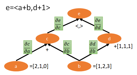
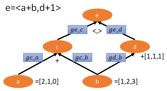
在 Tensorflow 中, tf.gradients 可以幫助計算 gradients. 舉例來說如果我們要計算 $\frac{\partial e}{\partial c}$, 我們只要這樣呼叫即可 ge_c=tf.gradients(ys=e,xs=c). 為了方便, 我們將 $\frac{\partial y}{\partial x}$ 在程式裡命名為 gy_x.

下面這段 codes 計算出上圖 5 個 edges 的 gradients:

import tensorflow as tf
import numpy as np
a = tf.placeholder(tf.float32, shape=(1,3))
b = tf.placeholder(tf.float32, shape=(1,3))
c = a + b
d = b + 1
e = tf.matmul(c,d,transpose_b=True)
ge_c, ge_d = tf.gradients(ys=e,xs=[c,d])
gc_a, gc_b = tf.gradients(ys=c,xs=[a,b])
gd_b = tf.gradients(ys=d,xs=b)
with tf.Session() as sess:
    sess.run(tf.global_variables_initializer())
    gec, ged, gca, gcb, gdb = sess.run([ge_c, ge_d, gc_a, gc_b, gd_b],feed_dict={a:[[2,1,0]],b:[[1,2,3]]})
    print('ge_c={}\nge_d={}\ngc_a={}\ngc_b={}\ngd_b={}'.format(gec, ged, gca, gcb, gdb))

計算結果為

ge_c=[[ 2.  3.  4.]]
ge_d=[[ 3.  3.  3.]]
gc_a=[[ 1.  1.  1.]]
gc_b=[[ 1.  1.  1.]]
gd_b=[array([[ 1.,  1.,  1.]], dtype=float32)]

可以自己手算驗證一下, 結果當然是對的 (使用 Jacobian matrix 計算)

所以我們如果要得到 $\frac{\partial e}{\partial b}$, 我們只要算 ge_c*gc_b + ge_d*gd_b 就可以了. 不過這樣自己把相同路徑做相乘，不同路徑做相加, 太麻煩了! 其實有更好的方法.

對於同一條路徑做相乘, tf.gradients 有一個 arguments 是 grad_ys 就可以很容易做到.

tf.gradients(ys=,xs=,grad_ys=)

以下圖來說明

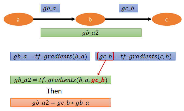
但事實上根本也不用這麼麻煩, 除非是遇到很特殊的狀況, 否則我們直接呼叫 tf.gradients(c,a), tensorflow 就會直接幫我們把同樣路徑的 gradients 做相乘, 不同路徑的 gradients 結果做相加了! 所以上面就直接呼叫 tf.gradients(c,a) 其實也就等於 gb_a2 了.

最後回到開始的 e=<a+b,b+1> 的範例, 如果要計算 $\frac{\partial e}{\partial b}$, 照原本提供的 codes 需要計算三條路徑各自相乘後再相加, 其實只要直接呼叫 ge_b=tf.gradients(e,b) 就完成這件事了 (ge_c*gc_b + ge_d*gd_b)

MNIST 用計算圖譜計算 back propagation

DNN 的計算圖譜

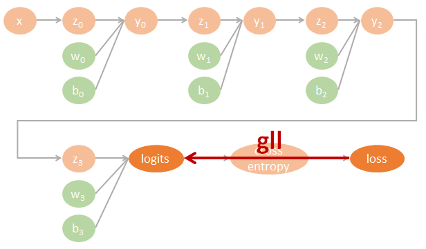
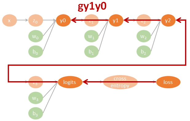
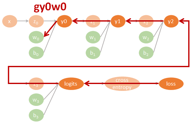
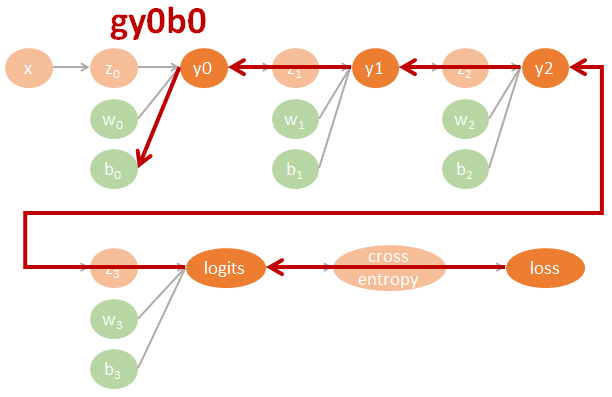
為了清楚了解 Neural network 的 backpropagation 如何用 computational graph 來計算 gradients 並進而 update 參數, 我們不使用 tf.optimizer 幫我們自動計算. 一個 3 layers fo MLP-DNN 的計算圖譜我們可以這樣表示:

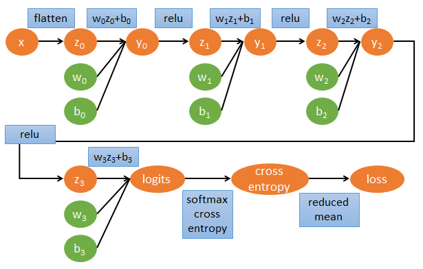
圖裡的參數直接對應了程式碼裡的命名, 因此可以很方便對照. 其中 tensorflow 裡參數的名字跟數學上的對應如下:

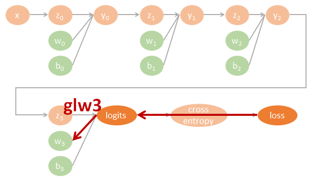
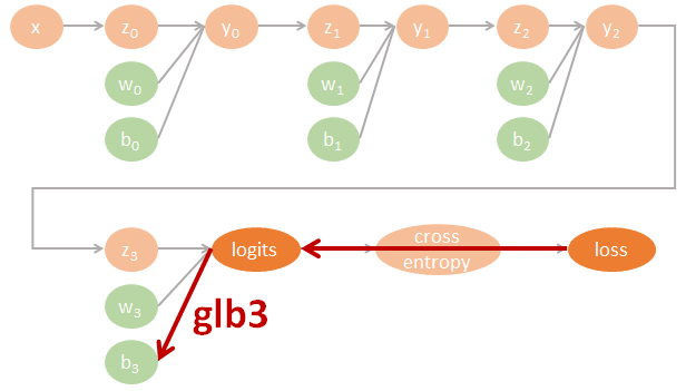
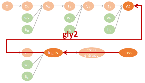
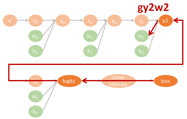
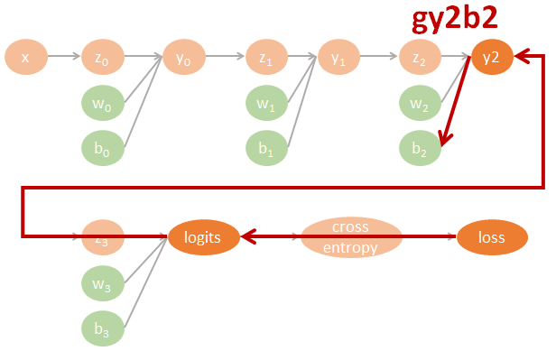
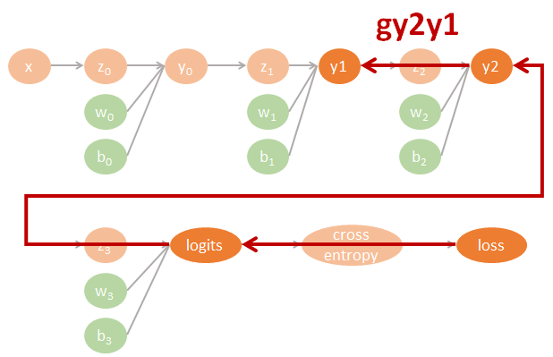
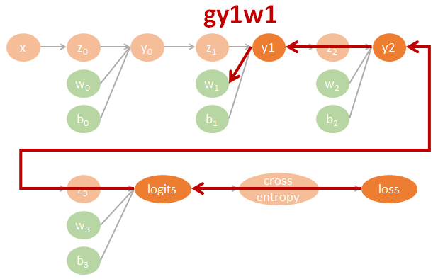
$$\begin{align} gll=\frac{\partial \mbox{loss}}{\partial \mbox{logits}} \\ gly2=\frac{\partial \mbox{logits}}{\partial y2}gll \\ gy2y1=\frac{\partial y2}{\partial y1}gly2 \\ gy1y0=\frac{\partial y1}{\partial y0}gy2y1 \\ (glw3,glb3)=(\frac{\partial \mbox{logits}}{\partial w3}gll,\frac{\partial \mbox{logits}}{\partial b3}gll) \\ (gy2w2,gy2b2)=(\frac{\partial y2}{\partial w2}gly2,\frac{\partial y2}{\partial b2}gly2) \\ (gy1w1,gy1b1)=(\frac{\partial y1}{\partial w1}gy2y1,\frac{\partial y1}{\partial b1}gy2y1) \\ (gy0w0,gy0b0)=(\frac{\partial y0}{\partial w0}gy1y0,\frac{\partial y0}{\partial b0}gy1y0) \end{align}$$

相對應的 tensorflow 代碼如下:

gll = tf.gradients(ys=loss,xs=logits)
gly2 = tf.gradients(ys=logits,xs=y2,grad_ys=gll)
gy2y1 = tf.gradients(ys=y2,xs=y1,grad_ys=gly2)
gy1y0 = tf.gradients(ys=y1,xs=y0,grad_ys=gy2y1)
glw3 = tf.gradients(ys=logits,xs=w3,grad_ys=gll)
glb3 = tf.gradients(ys=logits,xs=b3,grad_ys=gll)
gy2w2 = tf.gradients(ys=y2,xs=w2,grad_ys=gly2)
gy2b2 = tf.gradients(ys=y2,xs=b2,grad_ys=gly2)
gy1w1 = tf.gradients(ys=y1,xs=w1,grad_ys=gy2y1)
gy1b1 = tf.gradients(ys=y1,xs=b1,grad_ys=gy2y1)
gy0w0 = tf.gradients(ys=y0,xs=w0,grad_ys=gy1y0)
gy0b0 = tf.gradients(ys=y0,xs=b0,grad_ys=gy1y0)

用圖來表示為:

Tensorflow 程式碼

用上面一段的方式計算出所需參數的 gradients 後, update 使用最單純的 steepest descent, 這部分程式碼如下

update_w3 = tf.assign_add(w3,-rate*glw3[0])
update_b3 = tf.assign_add(b3,-rate*glb3[0])
update_w2 = tf.assign_add(w2,-rate*gy2w2[0])
update_b2 = tf.assign_add(b2,-rate*gy2b2[0])
update_w1 = tf.assign_add(w1,-rate*gy1w1[0])
update_b1 = tf.assign_add(b1,-rate*gy1b1[0])
update_w0 = tf.assign_add(w0,-rate*gy0w0[0])
update_b0 = tf.assign_add(b0,-rate*gy0b0[0])
training_operation = [update_w3, update_b3, update_w2, update_b2, update_w1, update_b1, update_w0, update_b0]

完整程式碼如下

import os
import numpy as np
import matplotlib.pyplot as plt
import tensorflow as tf
from tensorflow.contrib.layers import flatten
from tensorflow.examples.tutorials.mnist import input_data
from sklearn.utils import shuffle
"""
Data Loading
"""
dataPath='../dataset/MNIST_data/'
mnist = input_data.read_data_sets(dataPath, one_hot=True)
# read the images and reformat the image shape from [img_num,img_height,img_width] to [img_num,img_height,img_width,1]
img_width = 28
img_height = 28
images = mnist.train.images
img_num, _ = images.shape
images = np.reshape(images,(img_num,img_height,img_width))
images = images[...,np.newaxis]
print('(Input to CNN) Images with shape {}'.format(images.shape))
# read the labels
labels1Hot = mnist.train.labels
print('(Input to CNN) labels1Hot.shape = {}'.format(labels1Hot.shape))
labels = np.argmax(labels1Hot,axis=1)
labels = labels[...,np.newaxis]
print('labels.shape = {}'.format(labels.shape))
n_classes = len(np.unique(labels))
# load the validation set
images_valid = mnist.validation.images
img_num_valid = len(images_valid)
images_valid = np.reshape(images_valid,(img_num_valid,img_height,img_width))
images_valid = images_valid[...,np.newaxis]
labels1Hot_valid = mnist.validation.labels
print('Having %d number of validation images' % img_num_valid)
# plotting sample images
plt.figure(figsize=(15,5))
for i in np.arange(2*7):
    random_idx = np.random.randint(0,img_num)
    plt.subplot(2,7,i+1)
    plt.imshow(images[random_idx][...,0],cmap='gray')
    plt.title(labels[random_idx][0])
"""
First define the hyper-parameters
"""
# Hyper-parameters
EPOCHS = 30
BATCH_SIZE = 512
rate = 0.01
depth_list = [512, 256, 128]
cNum = 1
"""
Define the input output tensors
"""
# using one-hot decoding
x = tf.placeholder(tf.float32, (None, img_height, img_width, cNum))
one_hot_y = tf.placeholder(tf.int32, (None, n_classes))
#one_hot_y = tf.one_hot(y, n_classes)
"""
Define the graph and construct it
"""
z0 = flatten(x)
w0 = tf.get_variable('w0', shape=[img_width*img_height, depth_list[0]], initializer=tf.random_uniform_initializer(-0.1,0.1))
b0 = tf.get_variable('b0', [depth_list[0]], initializer=tf.zeros_initializer)
y0 = tf.nn.xw_plus_b(z0, w0, b0)
z1 = tf.nn.relu(y0)
w1 = tf.get_variable('w1', shape=[depth_list[0], depth_list[1]], initializer=tf.random_uniform_initializer(-0.1,0.1))
b1 = tf.get_variable('b1', [depth_list[1]], initializer=tf.zeros_initializer)
y1 = tf.nn.xw_plus_b(z1, w1, b1)
z2 = tf.nn.relu(y1)
w2 = tf.get_variable('w2', shape=[depth_list[1], depth_list[2]], initializer=tf.random_uniform_initializer(-0.1,0.1))
b2 = tf.get_variable('b2', [depth_list[2]], initializer=tf.zeros_initializer)
y2 = tf.nn.xw_plus_b(z2, w2, b2)
z3 = tf.nn.relu(y2)
w3 = tf.get_variable('w3', shape=[depth_list[2], n_classes], initializer=tf.random_uniform_initializer(-0.1,0.1))
b3 = tf.get_variable('b3', [n_classes], initializer=tf.zeros_initializer)
logits = tf.nn.xw_plus_b(z3, w3, b3)
cross_entropy = tf.nn.softmax_cross_entropy_with_logits(labels=one_hot_y,logits=logits)
loss = tf.reduce_mean(cross_entropy)
"""
Define gradients
"""
gll = tf.gradients(ys=loss,xs=logits)
gly2 = tf.gradients(ys=logits,xs=y2,grad_ys=gll)
gy2y1 = tf.gradients(ys=y2,xs=y1,grad_ys=gly2)
gy1y0 = tf.gradients(ys=y1,xs=y0,grad_ys=gy2y1)
glw3 = tf.gradients(ys=logits,xs=w3,grad_ys=gll)
glb3 = tf.gradients(ys=logits,xs=b3,grad_ys=gll)
gy2w2 = tf.gradients(ys=y2,xs=w2,grad_ys=gly2)
gy2b2 = tf.gradients(ys=y2,xs=b2,grad_ys=gly2)
gy1w1 = tf.gradients(ys=y1,xs=w1,grad_ys=gy2y1)
gy1b1 = tf.gradients(ys=y1,xs=b1,grad_ys=gy2y1)
gy0w0 = tf.gradients(ys=y0,xs=w0,grad_ys=gy1y0)
gy0b0 = tf.gradients(ys=y0,xs=b0,grad_ys=gy1y0)
update_w3 = tf.assign_add(w3,-rate*glw3[0])
update_b3 = tf.assign_add(b3,-rate*glb3[0])
update_w2 = tf.assign_add(w2,-rate*gy2w2[0])
update_b2 = tf.assign_add(b2,-rate*gy2b2[0])
update_w1 = tf.assign_add(w1,-rate*gy1w1[0])
update_b1 = tf.assign_add(b1,-rate*gy1b1[0])
update_w0 = tf.assign_add(w0,-rate*gy0w0[0])
update_b0 = tf.assign_add(b0,-rate*gy0b0[0])
training_operation = [update_w3, update_b3, update_w2, update_b2, update_w1, update_b1, update_w0, update_b0]
"""
Define accuracy evaluation
"""
# calculate the average accuracy by calling evaluate(X_data, y_data)
correct_prediction = tf.equal(tf.argmax(logits, axis=1), tf.argmax(one_hot_y, axis=1))
accuracy_operation = tf.reduce_mean(tf.cast(correct_prediction, tf.float32))
def evaluate(X_data, y_data):
    num_examples = len(X_data)
    total_accuracy = 0
    sess = tf.get_default_session()
    for offset in range(0, num_examples, BATCH_SIZE):
        batch_x, batch_y = X_data[offset:offset+BATCH_SIZE], y_data[offset:offset+BATCH_SIZE]
        accuracy = sess.run(accuracy_operation, feed_dict={x: batch_x, one_hot_y: batch_y})
        total_accuracy += (accuracy * len(batch_x))
    return total_accuracy / num_examples
    
"""
Run Session
"""
### Train your model here.
import time
if not os.path.isdir('./models'):
    os.makedirs('./models')
#saver = tf.train.Saver()
accumulate_time = 0.0
with tf.Session() as sess:
    sess.run(tf.global_variables_initializer())
    num_examples = img_num
    
    print("Training...")
    print()
    train_accuracy = np.zeros(EPOCHS)
    validation_accuracy = np.zeros(EPOCHS)
    for i in range(EPOCHS):
        stime = time.time()
        acc_train_accuracy = 0
        X_train, y_train = shuffle(images, labels1Hot)
        for offset in range(0, num_examples, BATCH_SIZE):
            end = offset + BATCH_SIZE
            batch_x, batch_y = X_train[offset:end], y_train[offset:end]
            sess.run(training_operation, feed_dict={x: batch_x, one_hot_y: batch_y})
        etime = time.time()
        accumulate_time += etime - stime
        validation_accuracy[i] = evaluate(images_valid, labels1Hot_valid)
        print("EPOCH {} ...".format(i+1))
        print("Validation Accuracy = {:.3f}".format(validation_accuracy[i]))
        print()
    print('Cost time: ' + str(accumulate_time) + ' sec.')

訓練結果如下:

EPOCH 1 ...
Validation Accuracy = 0.553
EPOCH 2 ...
Validation Accuracy = 0.698
EPOCH 3 ...
Validation Accuracy = 0.771
... 略
EPOCH 28 ...
Validation Accuracy = 0.936
EPOCH 29 ...
Validation Accuracy = 0.936
EPOCH 30 ...
Validation Accuracy = 0.936

這速度果然明顯比用 Adam 慢很多, 但至少說明了我們的確使用 Computational graph 的計算方式完成了 back propagation!

結論

Tensorflow 使用計算圖譜的框架來計算函數的 gradients, 一旦這樣做, 神經網路的 backprop 很自然了. 事實上, 所有流行的框架都這麼做, 就連 Kaldi 原先在 nnet2 不是, 但到 nnet3 也改用計算圖譜來實作.

Computational Graph

Verify with Tensorflow

MNIST 用計算圖譜計算 back propagation

DNN 的計算圖譜

Tensorflow 程式碼

結論

Reference