Coursera Stochastic Processes 課程筆記, 共十篇:
- Week 0: 一些預備知識
- Week 1: Introduction & Renewal processes (本文)
- Week 2: Poisson Processes
- Week3: Markov Chains
- Week 4: Gaussian Processes
- Week 5: Stationarity and Linear filters
- Week 6: Ergodicity, differentiability, continuity
- Week 7: Stochastic integration & Itô formula
- Week 8: Lévy processes
- 整理隨機過程的連續性、微分、積分和Brownian Motion
Week 1.2: Difference between various fields of stochastics
數學上的 stochastics 跟三個主要學科有關:
- Probability theory
- Mathematical statistics
- stochastic processes
用一個池子裡面的魚來當例子, 假設我們要分析某個時間點池子裡有多少魚, i.e. $N$ 條魚
Probability theory 就是找出這個 $N$ 的機率分布, 然後可以分析其 mean, variance …
而 mathematical statistics 是藉由一些統計實驗, 去估計出 $N$
舉例來說, 抓 $M$ 條魚做記號後放回池子. 然後一次實驗為抓 $n$ 條魚, 若發現有 $m$ 條做過記號, 則這個機率我們可以算出來:
$\mathcal{P}\{\#\text{marked}=m\}=(C_M^m\cdot C_{N-M}^{n-m})/C_N^n$
我們重複這個實驗 $q$ 次, 得到的做過記號的魚的次數為 ${m_1,m_2,…,m_q}$, 因此可以算出 log-likelihood:
$L(N)=\sum_{k=1}^q \log\mathcal{P}\{\#\text{marked}=m_k\}$
所以求解 $\arg\max_N L(N)$
對於 stochastic processes 我們也可以問同樣的問題: $N$ 是多少? 不過此時會多考慮 $N$ 隨著時間變化
Week 1.3: Probability space
建議先閱讀
[測度論] Sigma Algebra 與 Measurable function 簡介: https://ch-hsieh.blogspot.com/2010/04/measurable-function.html
[機率論] 淺談機率公理 與 基本性質: https://ch-hsieh.blogspot.com/2013/12/blog-post_7.html
課程使用兩個隨機實驗 (如同上面的參考連結):
- 從閉區間 $[0,1]$ 之中 任選一個數字
- 做 $n$ 次的丟銅板實驗
我們引用參考連結的定義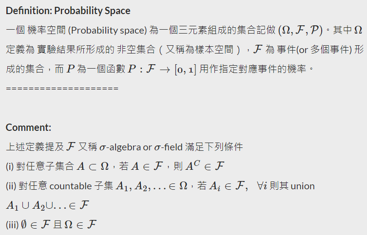
$\mathcal{F}$ 是一個 collection of subsets of $\Omega$, 也就是說每一個 element 都是一個 $\Omega$ 的 subset. 除此之外, 還必須是 $\sigma$-algebra.
$\sigma$-algebra 和 topology 定義可參考 https://www.themathcitadel.com/topologies-and-sigma-algebras/
所以一個 “事件” $A$ 是一個 subset of $\Omega$ (i.e. $A\subseteq\Omega$), 也是一個 element of $\mathcal{F}$, (i.e. $A\in\mathcal{F}$).
💡 注意 $A$ 是 subset of $\Omega$, 還不夠. $A$ 還必須從是 $\sigma$-algebra 的 $\mathcal{F}$ 裡面挑.
最後 $\mathcal{P}:\mathcal{F} \rightarrow [0,1]$ 此函數必須滿足以下公理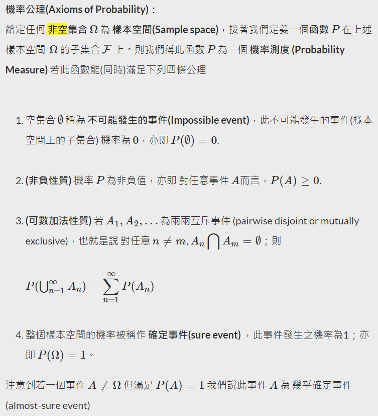
對比 measure 的定義, 相當於多出了一條 $P(\Omega)=1$, 所以 probability measure 是一個特殊的 measure
再對比 measure space 的定義, 差別只在於 probability space 用的 measure 為 probability measure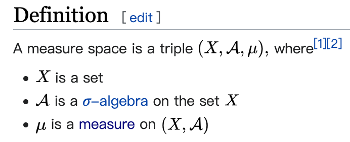
Week 1.4: Definition of a stochastic function. Types of stochastic functions.
首先 random variables 其實是一個 measurable function $\xi:\Omega\rightarrow\mathbb{R}$, 要搞清楚什麼是 measurable function 之前, 我們先要了解 Borel $\sigma$-algebra, Measurable Space 與 Measurable sets
$\sigma(\mathcal{E})$ 表示包含 $\mathcal{E}$ 的最小 $\sigma$-algebra, 且一定存在 (證明請參考該文章)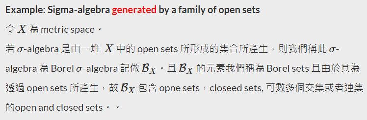
令 $X:=\mathbb{R}$, 則我們可以取所有 open sets 產生 Borel $\sigma$-algebra, 記做 $\mathcal{B}(\mathbb{R})$
$\mathcal{B}(\mathbb{R})$ 可以想成實數軸上包含所有 open sets 的最小 $\sigma$-algebra, 由 $\sigma$-algebra 定義知也包含 closed sets $[a,b]$, ${a}$, $(a,b]$, $[a,b)$, 以及上述這些的 countable union (complement)
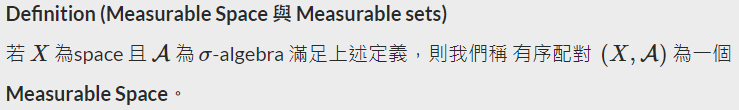
可稱 $\sigma$-algebra 中的元素為 measurable set
接著定義可測函數: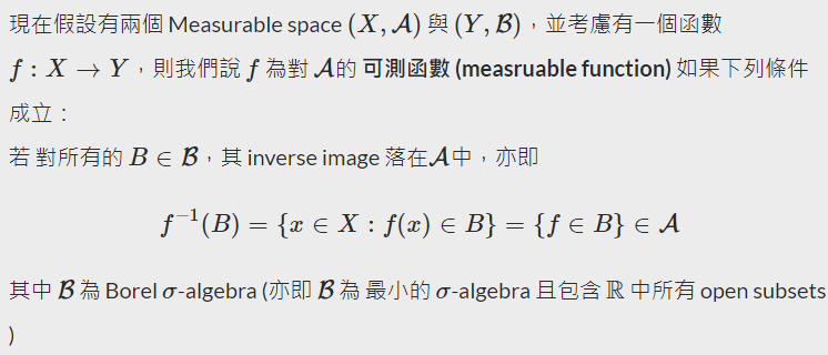
對於 $f$ 來說, 其 domain ($X$) and image ($Y$) spaces 都配備了對應的 $\sigma$-algebra $\mathcal{A},\mathcal{B}$
回到 probability space, $(\Omega, \mathcal{F}, \mathcal{P})$, 我們知道 $\mathcal{F}$ 是定義在 sample space $\Omega$ 的 $\sigma$-algebra, i.e. $(\Omega,\mathcal{F})$ 是 measurable space.
而 random variable $Z$ 其實是定義為由 $\Omega$ 映射到 $\mathbb{R}$ 的 measurable function. $\mathbb{R}$ 配備 $\mathcal{B}(\mathbb{R})$.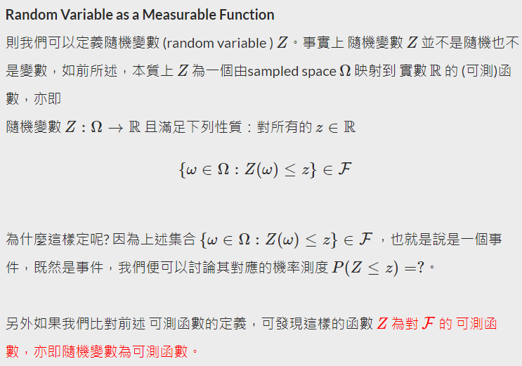
舉一個 Khan Academy 淺顯的例子, $X,Y$ 為兩個 r.v.s 分別把 outcomes 對應到 $\mathbb{R}$
$Y$ 的 outcomes 是
$\{(a_1,...,a_7):a_i\in \{\text{head,tail} \} \}$
共 $2^7$ 種可能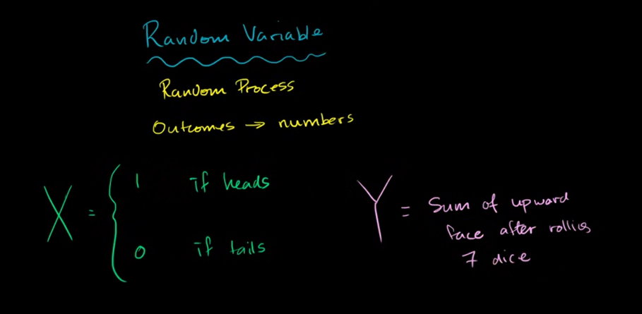
Mapping 到 $\mathbb{R}$ 後我們就可以算對應的機率, 例如
$\mathcal{P}(Y\leq30)$ or $\mathcal{P}(Y\text{ is even})$
而需要 r.v. 是 measurable function 的原因可以從這看出來, 因為我們要知道 pre-image:
$\{\omega:Y(\omega)\leq30\}$
也就是滿足這條件的 outcomes 集合, 必須要 $\in\mathcal{F}$. 所以它才會是個 “事件”
這是因為我們的 probability measure $\mathcal{P}:\mathcal{F}\rightarrow [0,1]$, 是定義在 $\mathcal{F}$ (事件的 $\sigma$-algebra) 上
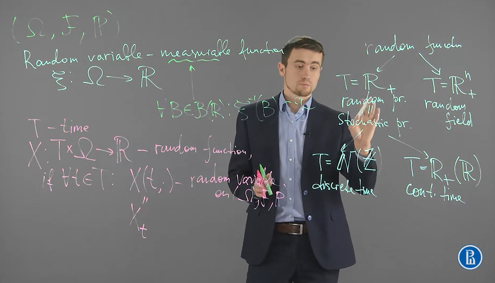
Week 1.5: Trajectories and finite-dimensional distributions
[Def]: Stochastic process
Stochastic process 是一個 mapping $X:T\times\Omega\rightarrow\mathbb{R}$, 而通常 $T=\mathbb{R}^+$, 且滿足:
$\forall t \in T$, we have $X_t=X(t,\cdot)$ is a random variable on probability space $(\Omega,\mathcal{F},\mathcal{P})$
[Def]: Trajectory (sample path, or path) of a stochastic process
對一個 stochastic process $X$ 來說, fixed $\omega\in\Omega$, 我們得到 $X(\cdot,\omega)$ 為 $T$ 的函數, 這就是 trajectory
所以 trajectory 就是對某一個 outcome $\omega$ 經過 random variable $X_t$ mapping 後的那個數值隨著時間的變化.
[Def]: Finite dimensional distributions
對一個 stochastic process $X$ 來說, 我們根據時間可以拿到 $n$ 個 random variables:
$(X_{t_1}, X_{t_2}, ..., X_{t_n})$, where $t_1, t_2,...,t_n \in \mathbb{R}$
在 probability theory 裡面都是將這 $n$ 個 r.v.s 視為獨立, 但在 stochastic processes 裡面不能. 這是很大的不同. 所以就算是 finite dimensional distribution, 在 stochastic processes 也是很挑戰的.
video 的試題:
Week 1.6: Renewal process. Counting process
可參考詳細解說: https://www.randomservices.org/random/renewal/Introduction.html
第一個事件發生的時間為 $T_1$, 第二個事件發生的時間為 $T_2$, …
每一個事件要隔多久發生都是從一個 random variable $X_i$ 決定的
因此我們會有一個 sequence of interarrival times, $X=(X_1,X_2,…)$
所以 sequence of arrival times 就會是 $T = (T_1, T_2, …)$, 其中
$T_n=\sum_{i=1}^nX_i$ , $n\in\mathbb{N}$
它們的關係用圖來看如下: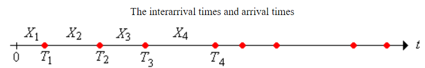
最後我們可以定義一個 random variable $N_t$ 表示到時間 $t$ 為止有多少個”事件”到達了:
$N_t=\sum_{n=1}^\infty \mathbf{1}(T_n\leq t)$, $t\in[0,\infty)$
其中 $\mathbf{1}(\cdot)$ 表示 indicator function.
又或者可以用課程上的定義:
$N_t=\arg\max_n\{T_n\leq t\}$
所以可以定義 counting process 為一個 random process $N=(N_t:t\geq 0)$
我們可以將 $N$ 這個 random processes 的 trajectory (path) 畫出來.
這個意思就是 fixed 一個 sample space 的值, 例如固定 $X’=(X_1=0.5,X_2=0.11,…)$, 然後對每個時間點的 $N_t$ 的值隨著時間畫出來. 我們會發現是如下的 increasing step function: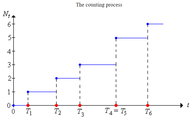
$T_n\leq t$ 意思就是 $n$ 個事件發生的時間比 $t$ 小. 等同於到時間 $t$ 為止至少有 $n$ 個事件已經發生, i.e. $N_t\geq n$
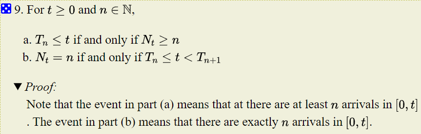
[Properties]: counting variables $N_t$ 與 arrival times $T_n$ 的關聯如下:
1. ${N_t\geq n}={T_n\leq t}$ or ${N_t\leq n}={T_n\geq t}$
2. $\{N_t=n\}=\{T_n\leq t\} \cap \{T_{n+1}>t\}$
Week 1.7: Convolution
我們有兩個互為獨立的 r.v.s $X\bot Y$, 且已知 $X\sim F_X$, $Y\sim F_Y$ (in c.d.f.) 或是寫成 $X\sim P_X$, $Y\sim P_Y$ (in p.d.f.).
$F_X$ and $F_Y$ 是 cumulated distribution function of $X$ and $Y$
$P_X$ and $P_Y$ 是 probability density function of $X$ and $Y$
$F_X(x)=P_X(X<x)$
則 convolution of two independent random variables 記做:
- $F_X\ast F_Y$ (convolution in terms of distribution function): $F_{X+Y}(x)=\int_\mathbb{R} F_X(x-y)dF_Y(y)$
- 或 $P_X \ast P_Y$ (convolution in terms of density function): $P_{X+Y}(x)=\int_\mathbb{R} P_X(x-y)P_y(y)dy$
💡 Convolution 同樣都是用 $\ast$ 表示, 但根據是 c.d.f. or p.d.f. 會有不同定義, 然而兩者為等價
把 convolution 擴展到 $n$ 個 i.i.d. r.v.s $\{X_1,X_2,...,X_n\}$, 其中 $X_i \sim F$, 則:
$S_n=X_1+...+X_n\sim {\color{orange}{F^{n\ast}=\underbrace{F\ast ...\ast F}_\text{n times}}}$
注意到這裡的 convolution, $\ast$, is in terms of distribution function
有幾個特性:
- $F^{n\ast}(x)\leq F^n(x)$, if $F(0)=0$
這是因為
$$\{X_1 + ... + X_n \leq x\}\subseteq\{X_1\leq x, ..., X_n\leq x\} \\ \therefore P\{X_1 + ... + X_n \leq x\}\leq \prod_{i=1}^n P\{X_i\leq x\} \\ =F^{n\ast}(x)\leq \prod_{i=1}^n F(x)=F^n(x)$$ - $F^{n\ast}(x)\geq F^{(n+1)\ast}(x)$
這是因為$\{X_1 + ... + X_n \leq x\}\supseteq\{X_1 + ... + X_n + X_{n+1} \leq x\}$
[Thm] Expectation of counting process equals to renewal function $\mathcal{U}(t)$:
考慮 renewal process: $T_n=T_{n-1}+X_n$, 且 $X_1,X_2,…$ are i.i.d. r.v.s with distribution function $F$.
$\mathcal{U}(t):=\sum_{n=1}^\infty F^{n\ast}(t) < \infty$
課程略過證明. 此定理告訴我們該序列收斂.
$F^{n\ast}(t)$ 的意思是 $n$ 個 i.i.d. r.v.s 相加的 CDF, i.e. $P(X_1+…+X_n\leq t)=P(T_n\leq t)$, 而在 renewal process 指的就是 arrival time $P(T_n\leq t)$, i.e. 到時間 $t$ 為止至少有 $n$ 個事件已經發生的機率.然後 $\sum_{n=1}^\infty$ 有那種把所有可能的情況都考慮進去的意思, 因此 $\mathcal{U}(t)$ 可能會跟到時間 $t$ 為止發生”事件”的次數的期望值 ($\mathbb{E} N_t$) 有關. 而事實上就是.
$\mathcal{U}(t)$ 稱 renewal function
$\mathbb{E} N_t = \mathcal{U}(t)$
$$\mathbb{E}N_t = \mathbb{E}\left[ \#\{n:T_n\leq t\} \right] =\mathbb{E}\left[ \sum_{n=1}^\infty \mathbf{1}(T_n\leq t) \right] \\ =\sum_{n=1}^\infty \mathbb{E}\left[ \mathbf{1}(T_n\leq t) \right] =\sum_{n=1}^\infty P(T_n\leq t) =\sum_{n=1}^\infty F^{n\ast}(t)$$
雖然 $\mathbb{E} N_t = \mathcal{U}(t) =\sum_{n=1}^\infty F^{n\ast}(t)$ 我們可以明確寫出來, 但對於 $F$ 是比較 general form 的話, 幾乎很難算出來. 因為要算 convolution, 又要求 sequence 的 limit.
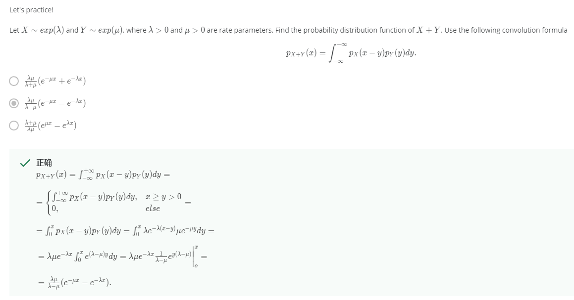
課程試題: 附上 exponential distributino 定義
Week 1.8: Laplace transform. Calculation of an expectation of a counting process-1
[Def]: Laplace transform
Given $f:\mathbb{R}^+\rightarrow\mathbb{R}$, Laplace transform 定義為如下積分:
$\mathcal{L}_f(s)=\int_{x=0}^\infty e^{-sx}f(x)dx$
有幾個主要的 properties:
- 令 $f$ 是 p.d.f. of some random variable $\xi$
則 $\mathcal{L}_f(s)=\mathbb{E}\left[ e^{-s\xi} \right]$ 給定任兩個 functions (不一定要是 p.d.f. or c.d.f.) $f_1$, $f_2$, 則 $\mathcal{L}_{f_1\ast f_2}(s)=\mathcal{L}_{f_1}(s)\cdot\mathcal{L}_{f_2}(s)$
$$\mathcal{L}_f(s)=\int_{x=0}^\infty e^{-sx}\left(\int_{y=0}^\infty f_1(x-y)f_2(y)dy\right)dx \\ =\int_{y=0}^\infty\left(\int_{x=0}^\infty e^{-sx}f_1(x-y)dx\right)f_2(y)dy \\ =\int_{y=0}^\infty\left( e^{-sy}\int_{x-y=y}^\infty e^{-s(x-y)}f_1(x-y)d(x-y) \right) f_2(y)dy \\ =\mathcal{L}_{f_1}(s)\cdot\int_{y=0}^\infty e^{-sy} f_2(y)dy = \mathcal{L}_{f_1}(s)\cdot\mathcal{L}_{f_2}(s)$$
其中 $\ast$ 是 convolution in terms of density
[Proof]:
Let $f(x)=f_1(x)*f_2(x)$ 則令 $F$ 是 c.d.f. 且 $F(0)=0$, $p=F’$ is p.d.f., 則:
$\mathcal{L}_F(s)=\frac{\mathcal{L}_p(s)}{s}\\$[Proof]: 使用分部積分, integration by part
$$l.h.s.=-\int_{\mathbb{R}^+}F(x)\frac{d(e^{-sx})}{s} = -\left[F(x)e^{-sx}/s\right]|_{x=0}^\infty+\frac{1}{s}\int_{\mathbb{R}^+}e^{-sx}dF(x) \\ = 0+\frac{1}{s}\int_{\mathbb{R}^+}p(x)e^{-sx}dx = r.h.s.$$
[Example 1]: 令 $f(x) = x^n$, 求 $\mathcal{L}_f(s)$
[sol]: 也是使用分部積分, integration by part
$$\mathcal{L}_{x^n}(s) = \int_{\mathbb{R}^+}x^n e^{-sx}dx =-\int_{\mathbb{R}^+}x^n\frac{d(e^{-sx})}{s} \\
= \frac{n}{s} \int_{\mathbb{R}^+}x^{n-1} e^{-sx}dx=...\\
=\frac{n}{s}\cdot\frac{n-1}{s}\cdot...\cdot\frac{1}{s}\int_{\mathbb{R}^+}e^{-sx}dx \\
=\frac{n!}{s^n}\cdot\left[ -\left.\frac{1}{s}e^{-sx} \right |_0^\infty \right] = \frac{n!}{s^{n+1}}$$
[Example 2]: 令 $f(x) = e^{ax}$, 求 $\mathcal{L}_f(s)$
[sol]: 答案為 $\mathcal{L}_{e^{ax}}(s)=\frac{1}{s-a}$, if $a<s$
略…
Week 1.9: Laplace transform. Calculation of an expectation of a counting process-2
現在我們要來計算 $\mathbb{E}N_t$, 回顧一下 $N_t$ 是一個 r.v. 表示到時間 $t$ 為止有多少個事件到達了
而我們也證明了 $\mathbb{E} N_t = \mathcal{U}(t) =\sum_{n=1}^\infty F^{n\ast}(t)$, 現在我們在仔細分析一下
$$\mathbb{E}N_t=\mathcal{U}(t)=\sum_{n=1}^\infty F^{n\ast}(t) \\
= F(t) + \left( \sum_{n=1}^\infty F^{n\ast} \right) \ast F(t) \\
= F(t) + \mathcal{U}(t)\ast F(t)$$
因此我們得到: $\mathcal{U}=F+\mathcal{U}\ast F$, 其中 convolution, $\ast$, is in terms of distribution function
然後我們對等號兩邊套用 Laplace transfrom, 但是我們注意到 Laplace transfrom 套用的 convolution 必須是 density function, 因此要轉換
其實我們從定義可以知道 $\mathcal{U}\ast_{cdf}F=\mathcal{U}\ast_{pdf}p$
已知 $p=F’$
$\int_{\mathbb{R}}\mathcal{U}(x-y)dF(y) = \int_{\mathbb{R}}\mathcal{U}(x-y)p(y)dy$
所以
$\mathcal{U}=F+\mathcal{U}\ast_{cdf} F = F+\mathcal{U}\ast_{pdf} p$, 然後就可以套用 Laplace transfrom, 並利用上面提到的 properties 2 & 3
$$\mathcal{L}_\mathcal{U}(s) = \mathcal{L}_F(s) + \mathcal{L}_\mathcal{U}(s) \cdot \mathcal{L}_p(s) \\
=\frac{\mathcal{L}_p(s)}{s} + \mathcal{L}_\mathcal{U}(s) \cdot \mathcal{L}_p(s)$$
因此
$\mathcal{L}_\mathcal{U}(s) = \frac{\mathcal{L}_p(s)}{s(1-\mathcal{L}_p(s))} \ldots (\star)$
所以雖然無法直接計算出 $\mathbb{E} N_t = \mathcal{U}(t)$, 但我們可以迂迴地透過以下三個步驟來估計:
- 從 $F$ 算出 $\mathcal{L}_p$
- 利用 $(\star)$ 從 $\mathcal{L}_p$ 算出 $\mathcal{L}_\mathcal{U}$
- 反推什麼樣的 $\mathcal{U}$ 會得到 $\mathcal{L}_\mathcal{U}$, 這一步是最困難的
下一段課程將會給出一個如何使用上面三步驟的範例
Week 1.10: Laplace transform. Calculation of an expectation of a counting process-3
[Example]: 假設我們有一個 renewal process, $S_n=S_{n-1}+\xi_n$
其中 $\xi_1, \xi_2, ... \sim p(x)=\frac{e^{-x}}{2}+e^{-2x}$
我們要如何計算 $\mathbb{E}N_t$?, 我們使用上面所述的三步驟:
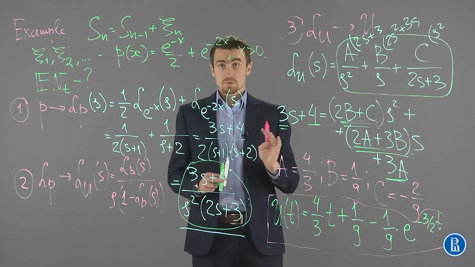
在最後一步的時候我要需要找出
什麼樣的 $\mathcal{U}(t)$ 會有 $\mathcal{L}_\mathcal{U}(s)=\frac{1}{s}$? Ans: $1$
什麼樣的 $\mathcal{U}(t)$ 會有 $\mathcal{L}_\mathcal{U}(s)=\frac{1}{s^2}$? Ans $t$
什麼樣的 $\mathcal{U}(t)$ 會有 $\mathcal{L}_\mathcal{U}(s)=\frac{1}{2s+3}$? Ans $\exp\{-\frac{3}{2}t\}$
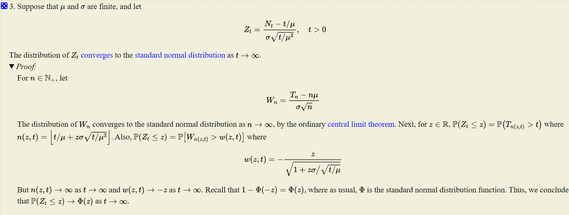
Week 1.11: Limit theorems for renewal processes
考慮一個 renewal process, $S_n=S_{n-1}+\xi_n$, 其中 $\xi_1,\xi_2,...$ are i.i.d. >0 almost surely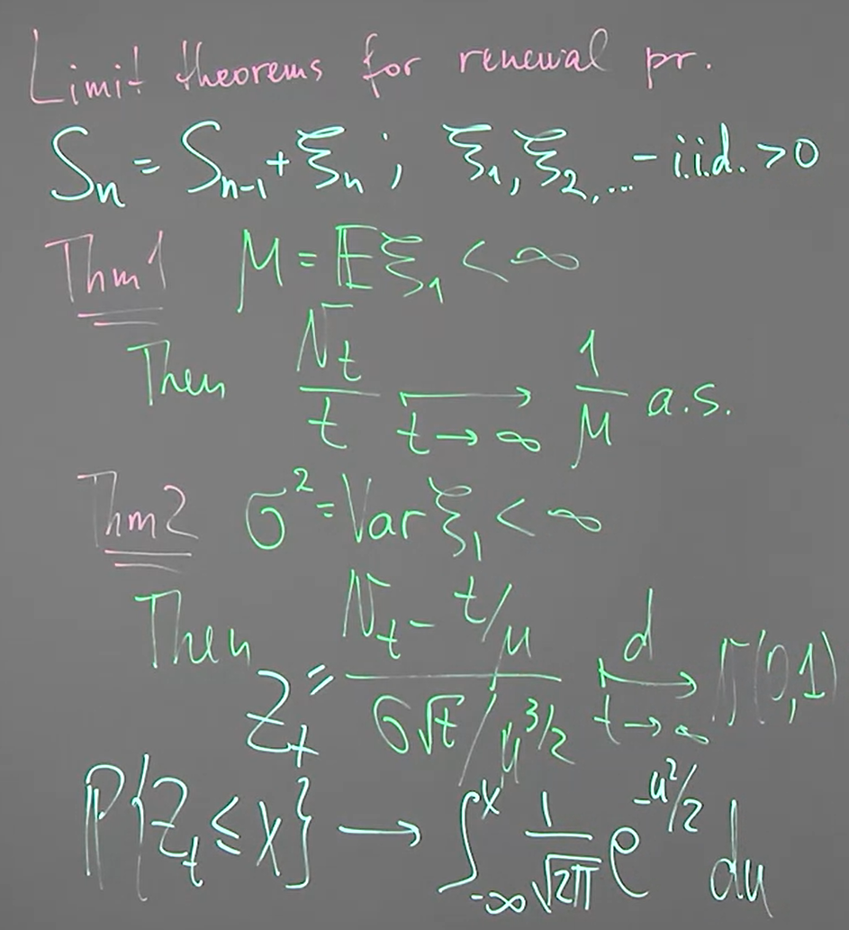
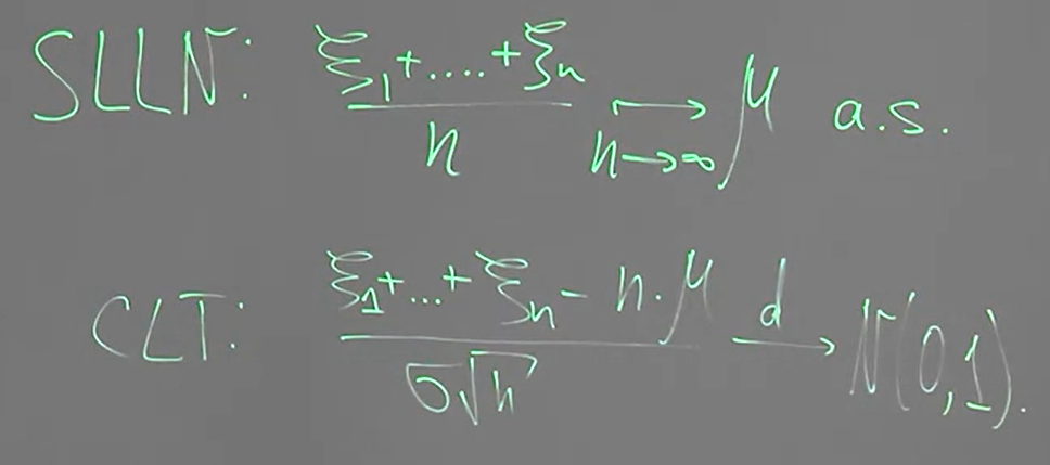
SLLN 為 Strong Law of Large Number; CLT 為 Central Limit Theorem
Thm1 直觀上可以理解, 因為 $N_t$ 表示到時間 $t$ 為止共有多少個事件發生了. 當 $t$ 很大的時候, 每單位時間發生的事件次數, i.e. $\frac{N_t}{t}$, 應該會十分接近頻率, i.e. $\frac{1}{\mu}$
Thm2 就不好直接理解了, 其中 $\xrightarrow[]{d}$ 表示 convergence in distribution. 注意到 $\frac{1}{\mu}$ 表示單位時間是間發生的次數, 所以乘上 $t$ 就是事件發生的次數, 注意到這是期望值, 而 $N_t$ 是發生次數的 random variable. 因此可以想像 mean 應該就是 $t/\mu$. 困難的是 variance 是什麼, 以及這剛好會 follow normal distribution.
而這兩個分別跟 SLLN (Strong Law of Large Number) and CLT (Central Limit Theorem) 相關. 以下給出證明
Thm1 的證明: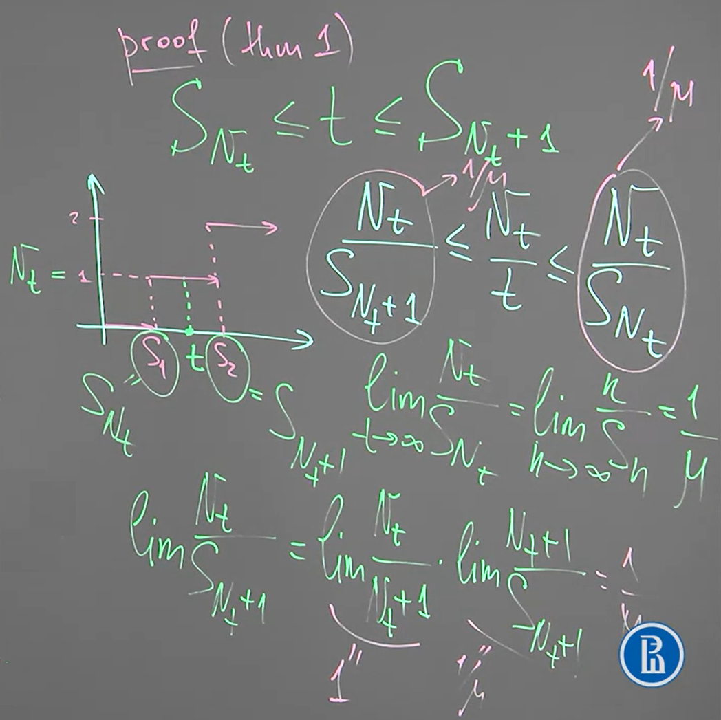
Thm2 的證明: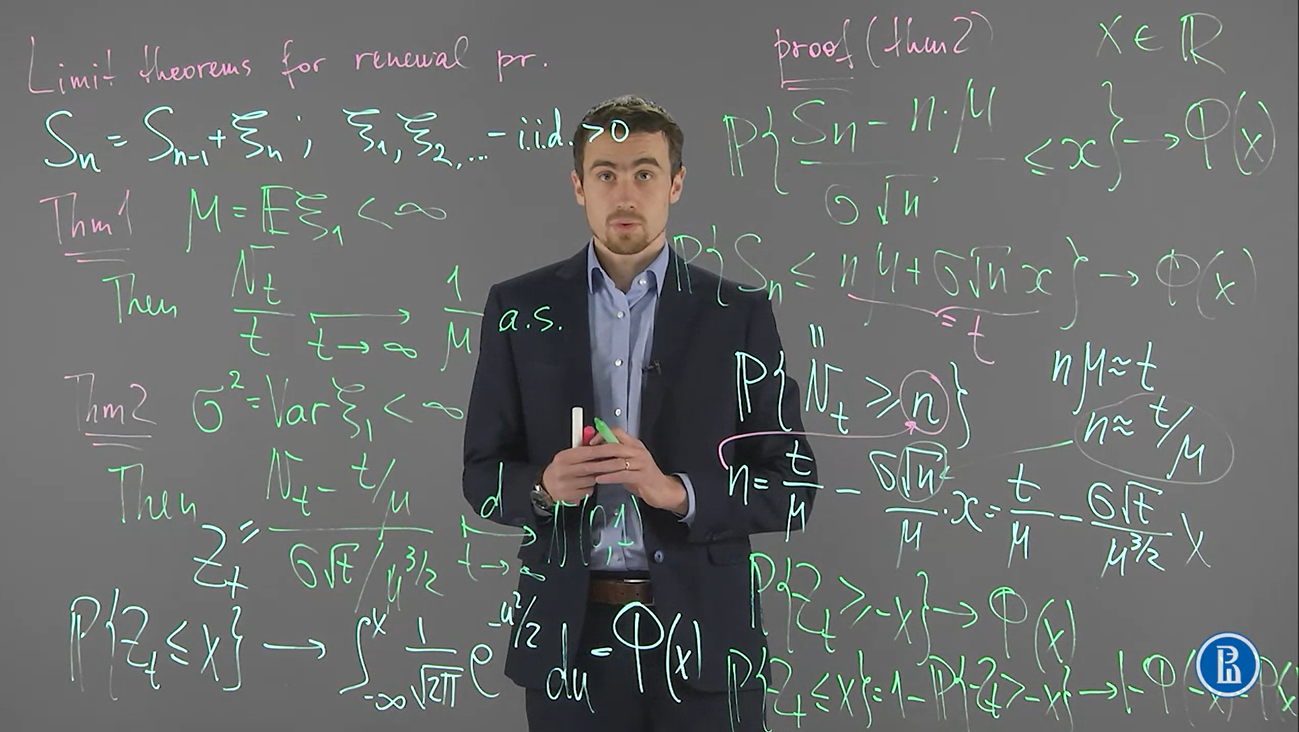
開頭的第一行:
$\mathcal{P}\left\{ \frac{\xi_1 + \xi_2 + ... + \xi_n -n\cdot\mu}{\sigma\sqrt{n}} \leq x \right\} = \mathcal{P}\left\{ \frac{S_n-n\cdot\mu}{\sigma\sqrt{n}} \leq x \right\}$
是從 CLT 出發
第二行到第三行用到了, $\mathcal{P}\left\{ S_n\leq t \right\} = \mathcal{P}\left\{ N_t \geq n \right\}$
然後由 $t=n\mu+\sigma\sqrt{n}x\Rightarrow n=\frac{t}{\mu}-\frac{\sigma\sqrt{n}}{\mu}x$ 並將 $n \approx t/\mu$ 帶入 r.h.s. 得到
$n=\frac{t}{\mu}-\frac{\sigma\sqrt{t}}{\mu^{3/2}}x$, 然後代回到 $\mathcal{P}\left\{ N_t \geq n \right\}$, 再整理一下得到最後一行
證明最後一行是 (被擋到):
$\mathcal{P}\left\{ Z_t \leq x \right\} = \mathcal{P}\left\{ Z_t > -x \right\} \rightarrow 1-\Phi(-x) = \Phi(x)$
或可以參考 https://www.randomservices.org/random/renewal/LimitTheorems.html 的 The Central Limit Theorem