Coursera Stochastic Processes 課程筆記, 共十篇:
- Week 0: 一些預備知識
- Week 1: Introduction & Renewal processes
- Week 2: Poisson Processes
- Week3: Markov Chains
- Week 4: Gaussian Processes
- Week 5: Stationarity and Linear filters (本文)
- Week 6: Ergodicity, differentiability, continuity
- Week 7: Stochastic integration & Itô formula
- Week 8: Lévy processes
- 整理隨機過程的連續性、微分、積分和Brownian Motion
Week 5.1-2: Two types of stationarity
[Strictly Stationary Def]:
$X_t$ is (strictly) stationary if $\forall(t_1,...,t_n)\in\mathbb{R}_+^n,\forall h>0$
$(X_{t_1+h},...,X_{t_n+h})=^d (X_{t_1},...,X_{t_n})$
Finite dimenstional distributions are invariant in shift in time
[Weakly Stationary Def]:
$X_t$ is (weakly) stationary, if $\forall t,s\in \mathbb{R}_+,\forall h>0$
$$m(t)=\mathbb{E}X_t=const \\
K(t,s)=Cov(X_t,X_s)=K(t+h,s+h)$$
存在 function $\gamma:\mathbb{R}\rightarrow\mathbb{R}$ (auto-covariance function) such that
$K(t,s)=\gamma(t-s)$
Shift in time 不變的只有 mean 和 covariance
Weak stationarity 也稱 second order stationarity 或 wide sense stationarity (WSS)
[Properties of Auto-covariance $\gamma(\cdot)$]:
1. $\gamma(0)\geq0$
$\gamma(0)=Cov(X_t,X_t)=Var(X_t)\geq0,\forall t\geq0$
2. $|\gamma(t)|\leq\gamma(0)$
$$|\gamma(t)|=|Cov(X_t,X_0)|\leq\sqrt{Var(X_t)}\sqrt{Var(X_0)} \\
= \sqrt{Cov(X_t,X_t)}\sqrt{Cov(X_0,X_0)} \\
= \sqrt{\gamma(t-t)}\sqrt{\gamma(0-0)}=\gamma(0)$$
3. $\gamma$ is even
$\gamma(t)=Cov(X_t,X_0)=Cov(X_0,X_t)=\gamma(-t)$
[Statements btw Strictly and Weakly Stationarity]:
1. We assume $\mathbb{E}X_t^2<\infty$, then $X_t$ is strictly stationary $\Longrightarrow$ $X_t$ is weakly stationary
2. $X_t$ is Gaussian process, then $X_t$ is strictly stationary $\Longleftrightarrow$ $X_t$ is weakly stationary
[Stationary of White Noise Process? Is Weak]:
$X_t,t=\pm1,\pm2,…$ is called white noise process, $WN(0,\sigma^2)$, if
$$\mathbb{E}X_t=0, Var(X_t)=\sigma^2 \\
Cov(X_t,X_s)=0,\forall t\neq s$$
i.e.
$m(t)=0,\gamma(0)=\sigma^2,\gamma(t)=0,\forall t>0$
or
$$\mathbb{E}X_t=0\\
K(t,s)=\sigma^2\mathbf{1}\{t=s\}=\gamma(t-s) \\
\therefore\gamma(x)=\sigma^2\mathbf{1}\{x=0\}$$
以上都是相同意思
$WN(0,\sigma^2)$ 可以看出是 weakly stationary, 通常情況下不一定是 strictly stationary, 因為根據定義只看 mean and covariance. 但有些情況會是 strict, 如:
- $X_1,X_2,…$ are i.i.d. noise
- $X_t$ is a Gaussian process (因為此時 strictly if and only if weakly)
[Stationary of Random Walk Process? Not Weak/Strict]:
$S_n=S_{n-1}+\xi_n$ where $\xi_1,\xi_2,...$ are i.i.d. with
$$\xi=\left\{
\begin{array}{rl}
1, & p \\
-1, & 1-p
\end{array}
\right.$$
Also assume $S_0=0$
知道 $S_n=\xi_1+…+\xi_n$, 計算一下 expectation
$\mathbb{E}S_n=n\mathbb{E}\xi_1=n(2p-1)$
所以如果 $p\neq\frac{1}{2}$, 則 $\mathbb{E}S_n$ depends on $n$
所以 $S_n$ 不是 weakly stationary (因此也一定不是 strictly)
所以我們 focus 在 $p=\frac{1}{2}$, 接著計算 covariance, for $n>m$
$$K(n,m)=Cov(S_m+\xi_{m+1}+...+\xi_n, S_m) \\
= Cov(S_m,S_m)+Cov(\xi_{m+1}+...+\xi_n,S_m) \\
=m\cdot Var(\xi_1)+0=\min\{n,m\}Var(\xi_1)$$
所以 $K(n,m)$ 無法只用 $n-m$ 來表示, 因此 Random walk 不是 strictly/weakly stationary
[Stationary of Brownian Motion? Not Weak/Strict]:
$\mathbb{E}B_t=0$, and $Var(B_t)=t$. 且知道 $B_t-B_s\sim\mathcal{N}(0,t-s)$
$K(t,t)=Cov(B_t,B_t)=Var(B_t)=t$, $\because B_t\sim\mathcal{N}(0,t)$
所以不存在 $\gamma(t-s)=K(t,s)$, 因為我們看 $\gamma(0)$ 就知道不固定, $\gamma$ 不符合 function 定義
或可以從 $K(t+h,s+h)=?K(t,s)$ 觀察, 已知 Brownian motion $K(t,s)=\min\{t,s\}$
則 $K(t+h,s+h)\neq K(t,s)$
結論 Brownian motion is not weakly stationary (因此一定也不是 strictly)
[Stationary of Moving Average Process? Is Weak]:
$X_t\sim WN(0,\sigma^2)$. Given $a_1,…,a_q\in\mathbb{R};a_0=1$. Moving average $Y_t$ defined as:
$Y_t=X_t+a_1X_{t-1}+...+a_qX_{t-q}$
用 $MA(q)$ 表示
$\mathbb{E}Y_t=\mathbb{E}[X_t]+a_1\mathbb{E}[X_{t-1}]+...+a_q\mathbb{E}[X_{t-q}]=0$
$$K(t,s)=Cov\left(\sum_{j=0}^qa_jX_{t-j},\sum_{k=0}^qa_kX_{s-k}\right) \\
= \sum_{j=0}^q \sum_{k=0}^q a_ja_kCov(X_{t-j},X_{s-k}) \\
= \sum_{j=0}^q \sum_{k=0}^q a_ja_k \sigma^2\mathbf{1}\{t-s=j-k\}$$
因此可以看出 $K(t,s)$ 只跟 $t-s$ 有關
MA(1):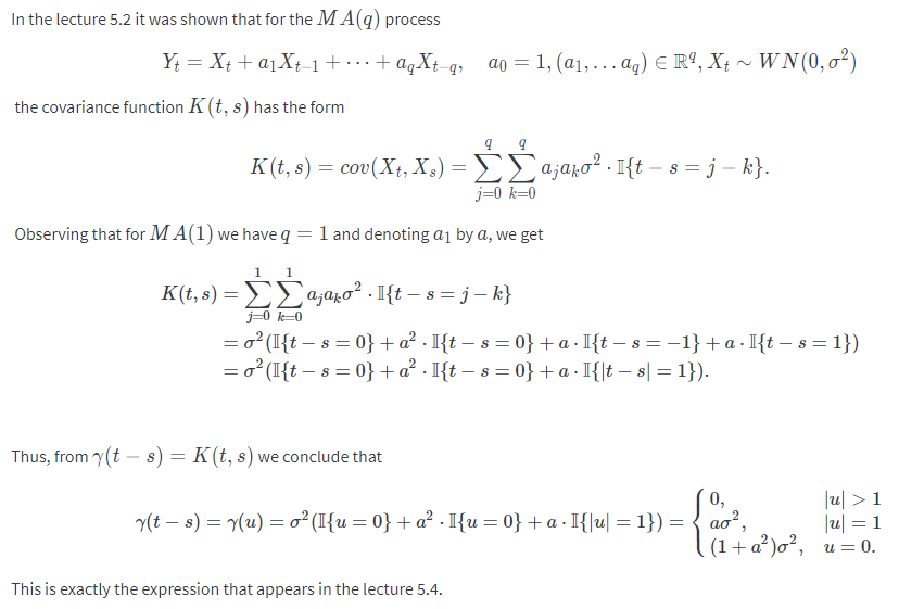
所以是 Weakly stationary
這個 moving average 是 FIR (linear), input $X_t$ 是 white noise, 所以為 weakly stationary. 由 weakly stationary 經過 linear filter 其 output 仍為 weakly stationary 可得到結論.
[Stationary of Autoregressive Model? Weak in Constraint]:
$\xi_t\sim WN(0,\sigma^2)$, we say that $Y_t$ is autoregressive model, $AR(p)$, if:
$Y_t=b_1Y_{t-1}+...+b_pY_{t-p}+\xi_t$
Also we assume $Cov(\xi_t,Y_s)=0,\forall t>s$
考慮 $AR(1)$:
$$Y_t=bY_{t-1}+\xi_t \\
=b(bY_{t-2}+\xi_{t-1})+\xi_t \\
= ... = \sum_{j=0}^\infty b^j\xi_{t-j}$$
明顯可以看出 $\mathbb{E}Y_t=0$, 接著計算 covariance:
$$K(t,s)=Cov(Y_t,Y_s)=\sum_{j,k=0}^\infty b^{j+k}\cdot Cov(\xi_{t-j},\xi_{s-k}) \\
= \sum_{j,k=0}^\infty b^{j+k} \cdot \sigma^2\cdot\mathbf{1}\{t-s=j-k\}$$
看起來 covariance 只跟 $t-s$ 有關, 但我們計算一下 $\gamma(0)=K(t,t)$:
$$t-s=0\Rightarrow K(t,t)=\sum_{k=0}^\infty b^{2k}\cdot \sigma^2 \\
\therefore K(t,t)<\infty\Leftrightarrow |b|<1$$
只有在 $|b|<1$ 的情況 variance 才收斂, 因此 weakly stationary 才成立
考慮 $AR(p)$, 課程說 $Y_t$ 一樣可以寫出 $\xi_t$ 的和, 找出所有根並在 norm<1 才收斂
這就是 IIR 的 poles 要在單位圓內
總之, autoregressive model 有條件地成為 weakly stationary
Week 5.3-4: Spectral density of a wide-sense stationary process
[Bochner–Khinchin Theorem]:
$\Phi:\mathbb{R}\rightarrow\mathbb{C}$, and $\Phi(u)$ is a characteristic function, i.e.
$\exists\xi$ random variable such that $\Phi(u)=\mathbb{E}[e^{iu\xi}]$
$\Longleftrightarrow$
1. $\Phi$ is continuous
2. $\Phi$ is positive semi-definite
$$\forall(z_1,...,z_n)\in\mathbb{C}^n,\forall(u_1,...,u_n)\in\mathbb{R}^n \\
\sum_{j,k=1}^n z_j\overline{z_k}\Phi(u_j-u_k)\geq0$$
3. $\Phi(0)=1$
[Bochner–Khinchin Theorem Alternative 1]:
如果只滿足 1. and 2. 則可以得到 $\exists\mu$ is some measure such that
$\Phi(u)=\int e^{iux}\mu(dx)$
$\mu$ 可以不必是 probability measure (但我們知道一定會有個 measure 滿足上式)
[Bochner–Khinchin Theorem Alternative 2]:
如果滿足 1. and 2. and 如下條件
$\int|\Phi(u)|du<\infty$
則 $\Phi:\mathbb{R}\rightarrow\mathbb{C}$, and $\Phi(u)$ is a characteristic function
i.e. 某個 r.v. $\xi$ 的 p.d.f. 為 $s(x)$ 的 Fourier transform
相比 alternative 1, 此時 measure $\mu$ 有 density $s(x)$
$\Phi(u)=\int e^{iux}s(x)dx$
💡 注意到課程的 Fourier transform 跟我們一般在訊號處理的有點不同, 課程的定義為:
$\mathcal{F}[g](u)=\int e^{iux}g(x)dx$
且課程的 spectral density 在訊號處理我們稱 “power” spectral density
[Spectral Density of Weakly Stationary Def]:
Let $X_t$ is weakly stationary 且 $\gamma:K(t,s)=\gamma(t-s)$
If $\gamma$ is continuous (本身已經是半正定) and $\int|\gamma(u)|du<\infty$
使用 Bochner–Khinchin Theorem Alternative 2 則 $\exists g(x)$ a density such that
$$\color{orange}{
\gamma(u)=\int_\mathbb{R} e^{iux}g(x)dx }\\
= \mathcal{F}[g](u) \text{ (i.e. Fourier transform of }g)$$
也等於
$$\color{orange}{
g(x)=\frac{1}{2\pi}\int_\mathbb{R} e^{-iux}\gamma(u)du }\\
= \frac{1}{2\pi}\mathcal{F}[\gamma](-x)$$
此時 $g(x)$ 稱為 $X_t$ 的 spectral density
在 discrete case 為
$$\color{orange}{
g(x)=\frac{1}{2\pi}\sum_{h=-\infty}^\infty e^{-ihx}\gamma(h)
}$$
在 WSS 條件下, auto-covariance $\gamma$ 就等同於特徵方程式了
(注意到特徵方程式為 pdf 的 Fourier transform)
[Examples]:
White noise, $WN(0,\sigma^2)$, $\gamma(u)=\sigma^2\cdot\mathbf{1}\{u=0\}$, 所以
$g(x)=\frac{\sigma^2}{2\pi}$
Moving average, $MA(1)$
$$\gamma(u)=\left\{
\begin{array}{rl}
0, & |u|>1 \\
a\sigma^2, & |u|=1 \\
(1+a^2)\sigma^2, & u=0
\end{array}
\right. \\
g(x)=\frac{\sigma^2}{2\pi}\left(1+a^2+a\cdot2\cos(x)\right)$$
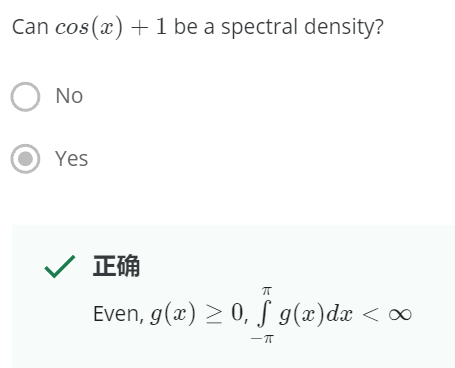
[Sufficient and Necessary Condition for a Function is a Spectral Density]:
A real-valued function $g(x)$ defined on $(-\pi,\pi]$
is a spectral density of a stochastic process $X_t$
if and only if
1. $g(x)\geq0$
2. $g(x)$ is even
3. $\int_{-\pi}^\pi g(x)dx<\infty$
用 “power” spectral density 來記憶, 因為是 power 所以 1. 2. 合理一定要
Week 5.5: Stochastic integration of the simplest type
[Stochastic Integrals Def]:
Given a Stochastic process $X_t$
Given partition $\Delta:a=t_0\leq t_1\leq ...\leq t_n=b$, $|\Delta|=\max\{t_k-t_{k-1}\},k=1,...,n$
If the following expectation converges to some value $A$ in mean square sense:
$$\mathbb{E}\left[
\left(
A - \sum_{k=1}^n X_{t_{k-1}}(t_k-t_{k-1})
\right)^2
\right]
\xrightarrow[|\Delta|\longrightarrow0]{} 0$$
Then we denote(define) the converged value $A$ as:
$\int_a^b X_t dt$
💡 參考課程 Week 7.1: Different types of stochastic integrals. Integrals of the type $∫ X_t dt$
[Existence of Stochastic Integral]:
$X_t:\mathbb{E}[X_t^2]<\infty$, if
1. $m(t)$ continuous
2. $K(t,s)$ continuous
Then the stochastic integral exists
$\int_a^b X_tdt<\infty$
要證明 $K(t,s)$ continuous, 其實只需要 check diagonal 項就可以
💡 只對 covariance function $K(t,s)$ 有這樣的特性, 我們再 Week 6.4 會證明
[Lemma]:
1. Stochastic process $X_t$. If $K(t,s)$ is continuous at $(t_0, t_0)$
then $X_t$ is continuous at $t_0$ (in mean square sense), that is
$\mathbb{E}[(X_t-X_{t_0})^2]\rightarrow0,\text{ as }t\rightarrow t_0$
2. On the other side, if $X_t$ is continuous at $t_0$ and $s_0$
then $K(t,s)$ is continuous at $(t_0,s_0)$, that is $K(t_0,s_0)$ is continuous
[Covariance Function is Continuous when Continuous on Diagonal]:
Covariance function $K(t,s)$ is continuous $\forall(t_0,s_0)$ $\Longleftrightarrow$
$K(t,s)$ is continuous $\forall(t_0,t_0)$
[Proof]:
$(\Longrightarrow)$: of course
$(\Longleftarrow)$:
$K(t,s)$ is continuous $\forall(t_0,t_0)$, 由 Lemma 1 知道 $X_t$ is countinuous $\forall t_0$
因此 $X_t$ is continuous $\forall t_0,s_0$, 由 Lemma 2 知道 $K(t_0,s_0)$ is countinuous $\forall t_0,s_0$
[Properties of Stochastic Integral]: assume integral exists
We assume integral is taken in an bounded interval $[a,b]$
1. Expectation of stochastic integral:
$\mathbb{E}\left[ \int X_tdt \right] = \int \mathbb{E}[X_t]dt$
課程老師說 apply Frobenius theorem 可得此結果. 看不懂 Frobenius theorem
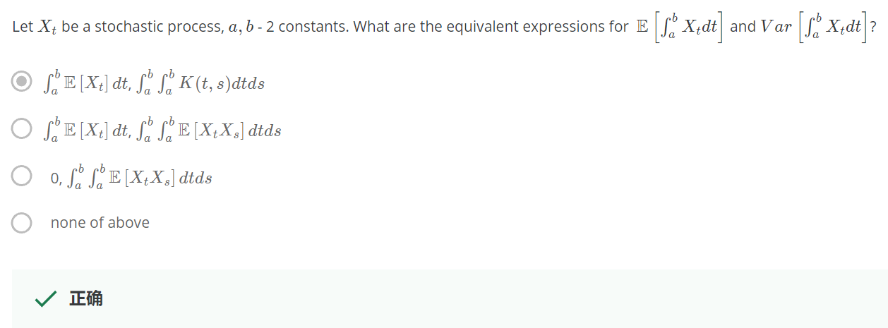
2. Expectation of squared stochastic integral:
$$\mathbb{E}\left[
\left(\int X_t dt\right)^2
\right] = \mathbb{E}\left[
\int\int X_t X_s dtds
\right] \\
= \int\int\mathbb{E}[X_tX_s]dtds$$
3. Variance of stochastic integral:
$$Var\left[
\int X_t dt
\right] = \mathbb{E}\left[
\left(\int X_t dt\right)^2
\right] - \left(\mathbb{E}\left[ \int X_tdt \right]\right)^2 \\
= \int_a^b\int_a^b K(t,s) dtds \\
\because\text{symmetric}= 2\int_a^b \int_a^s K(t,s) dtds$$
課程 pop up quiz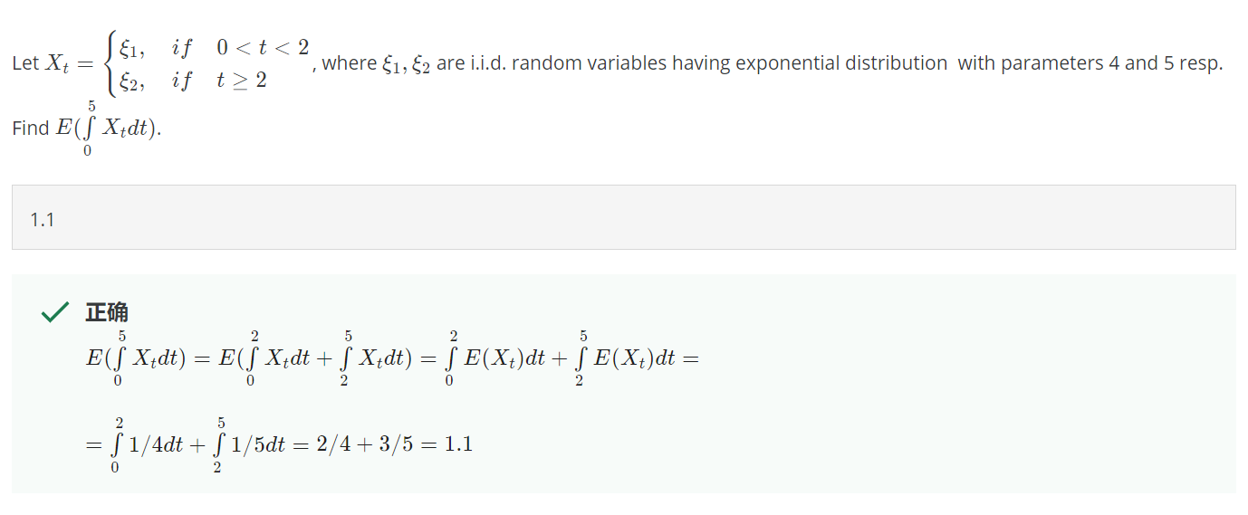
Week 5.6-8: Moving-average filters
Filter 就是把某個 stochastic process $X_t$ transform 到另一個 $Y_t$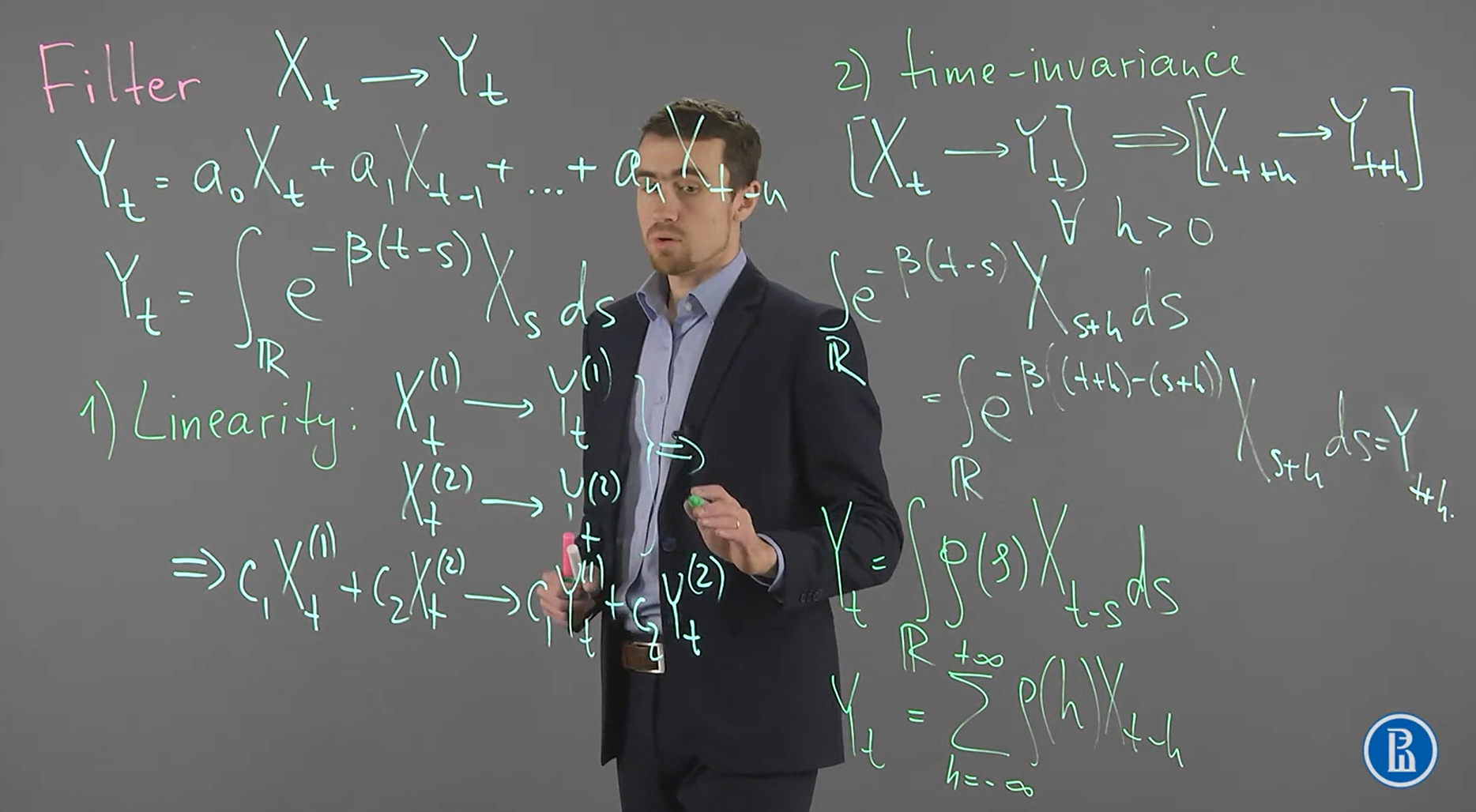
Filter 有 linearity and time-invariant 兩個重要 properties
課程舉兩個 filter 的例子 (第一個為 FIR, 第二個為 simplest stochastic integral)
$$\begin{align}
Y_t=a_0X_t+a_1X_{t-1}+...+a_nX_{t-n} \\
Y_t=\int_\mathbb{R} e^{-\beta(t-s)}X_sds
\end{align}$$
都具有上述 properties, 也很容易證
然後上圖右下角寫出 filtering 的 continuous and discrete 的數學式, 顯然這是 convolution
$$Y_t=\int_\mathbb{R}\rho(s)X_{t-s}ds \\
Y_t=\sum_{h=-\infty}^\infty \rho(h)X_{t-h}$$
[Spectral Density and Weakly Stationary by Linear Filter]:
$X_t$ is weakly stationary with $\mathbb{E}X_t=0$ and some spectral density $g(x)$.
$Y_t$ is linear filtered by $\rho(x)$ from $X_t$:
$Y_t=\int_\mathbb{R} \rho(s)X_{t-s}ds$
Then,
1. $Y_t$ is weakly stationary
2. Spectral density of $Y_t$:
$$\color{orange}{
g_Y(u)=g_X(u)\cdot|\mathcal{F}[\rho](u)|^2
}$$
here the Fourier transform of $\rho$ is:
$\mathcal{F}[\rho](u)=\int_\mathbb{R} e^{-iux}\rho(x)dx$
[Proof 1. weakly stationary]:
觀察 expectation and covariance functions 是否符合 weakly stationary
$\mathbb{E}[Y_t]=\int_\mathbb{R}\rho(s)\mathbb{E}[X_{t-s}]ds=0$
因為 $\mathbb{E}[Y_t]=0$, 所以 $K(t,s)=Cov(Y_t,Y_s)=\mathbb{E}[Y_tY_s]$, then
$$K_Y(t_1,t_2)=\mathbb{E}\left[
\int_\mathbb{R}\rho(s_1)X_{t_1-s_1}ds_1 \cdot \int_\mathbb{R}\rho(s_2)X_{t_2-s_2}ds_2
\right] \\
=\int_\mathbb{R}\int_\mathbb{R}
\rho(s_1)\rho(s_2)\mathbb{E}[X_{t_1-s_1}X_{t_2-s_2}]
ds_1ds_2 \\
=\int_\mathbb{R}\int_\mathbb{R}
\rho(s_1)\rho(s_2)\gamma(
\color{orange}{t_2-t_1}
-(s_2-s_1))
ds_1ds_2 \\$$
所以只 depends on $t_2-t_1$, 所以 auto-covariance of $Y_t$ 存在如下:
$$\gamma_Y(x)=\int_\mathbb{R}\int_\mathbb{R}
\rho(s_1)\rho(s_2)\gamma(
x
-(s_2-s_1))
ds_1ds_2$$
Q.E.D.
[Proof 2. Spectral density of $Y_t$]:
由 proof 1 知道 $\gamma_Y(x)$ 改寫如下:
$$\gamma_Y(x)=\int_\mathbb{R}\rho(s_1)
\color{orange}{\int_\mathbb{R}\rho(s_2)\gamma((x+s_1)-s_2)ds_2}
ds_1 \\
=\int_\mathbb{R}\rho(s_1)
\color{orange}{[\gamma_X*\rho](x+s_1)}
ds_1 \ldots(\star)\\$$
定義 $\rho^o(x)=\rho(-x)$, 在把 $s_1$ 改寫成 $-s_1$, 則 $(\star)$ 變成:
$$\gamma_Y(x)=(\star)=\int_\mathbb{R}\rho^o(s_1)
[\gamma_X*\rho](x-s_1)
ds_1 \\
=[\gamma_X*\rho*\rho^o](x)\ldots(\square)$$
注意到 spectral density 跟 auto-covariance 的關係為 Fourier transform 的關係:
$g_Y(u)=\frac{1}{2\pi}\mathcal{F}[\gamma_Y](-u)$
所以對 $(\square)$ 兩邊取 Fourier transform 我們得到:
$$g_Y(u)=
\frac{1}{2\pi}\mathcal{F}[\gamma_Y](-u)=\frac{1}{2\pi}\mathcal{F}[\gamma_X](-u)\cdot\mathcal{F}[\rho](-u)\cdot\mathcal{F}[\rho^o](-u) \\
=g_X(u)\cdot|\mathcal{F}[\rho](u)|^2$$
Q.E.D.
Let $X_t$ is weakly stationary, and it’s spectral density is $g_X(u)$. 我們想用 moving average $MA(2)$ 來預測當下這個時間點的 $X_t$:
$Y_n=a_1X_{n-1}+a_2X_{n-2}$
如何決定 $a_1,a_2$ 來使得預測最準 (in least square error sense):
$\mathbb{E}[(X_n-Y_n)^2]\rightarrow \min$
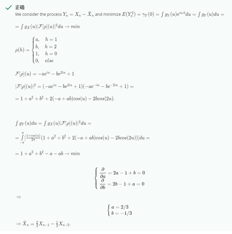
我們知道 $Z_n=X_n-Y_n=X_n-a_1X_{n-1}-a_2X_{n-2}$ 也是 weakly stationary, 因為過一個 linear filter $\rho(x)$:
$\rho(x)=\mathbf{1}\{x=0\}-a_1\mathbf{1}\{x=1\}-a_2\mathbf{1}\{x=2\}$
其 Fourier transform 為: $\mathcal{F}[\rho](u)=1-a_1e^{iu}-a_2e^{2iu}$
則 spectral density of $Z$ 為: $g_Z(u)=g_X(u)\cdot|\mathcal{F}[\rho](u)|^2$
所以問題等同於計算$\arg\min_{a_1,a_2} VarZ_n$
計算 $Var Z_n$ 如下
$$Var(Z_n)=K_Z(n,n)=\gamma_Z(0)\\
=\int e^{i\cdot u\cdot 0}g_Z(u)du \\
=\int g_X(u)\cdot|1-a_1e^{iu}-a_2e^{2iu}|^2 du \\
=\int g_X(u)\cdot(1-a_1e^{iu}-a_2e^{2iu})\cdot(1-a_1e^{-iu}-a_2e^{-2iu}) du \\
=...=\sum_{i,j=1}^2 B_{ij}a_ia_j + \sum_{i=1}^2 C_ia_i + D$$
所以最小化一個二次式即可求得最佳解 $a_1,a_2$
[Pop up Quiz]: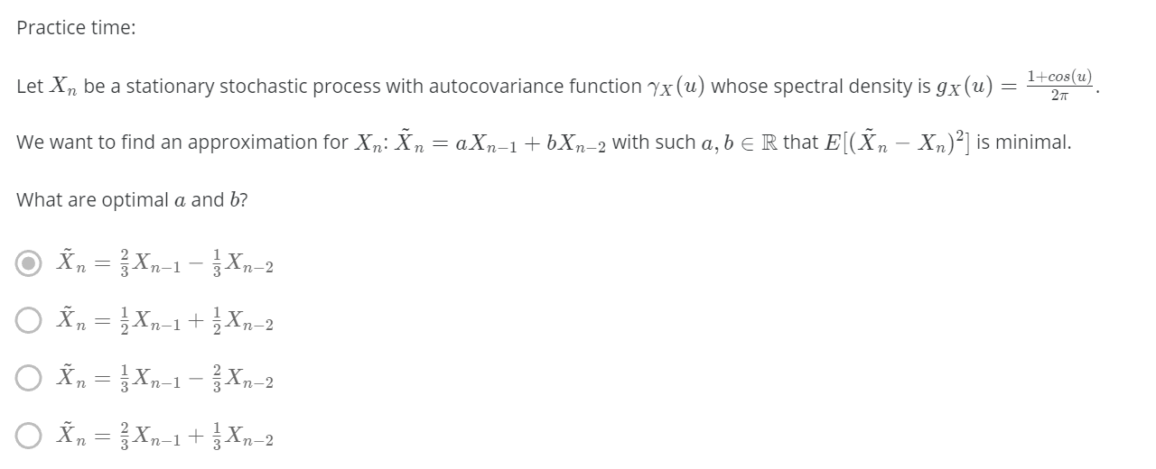
有點難算 XD 容易算錯