Coursera Stochastic Processes 課程筆記, 共十篇:
- Week 0: 一些預備知識
- Week 1: Introduction & Renewal processes
- Week 2: Poisson Processes (本文)
- Week3: Markov Chains
- Week 4: Gaussian Processes
- Week 5: Stationarity and Linear filters
- Week 6: Ergodicity, differentiability, continuity
- Week 7: Stochastic integration & Itô formula
- Week 8: Lévy processes
- 整理隨機過程的連續性、微分、積分和Brownian Motion
Week 2.1-4: Definition of a Poisson process as a special example of renewal process. Exact forms of the distributions of the renewal process and the counting process
Just a recap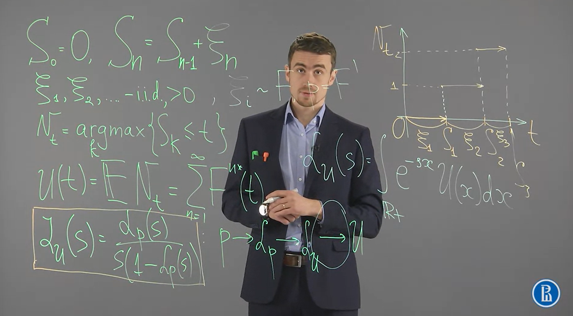
令我們有如上面所述的 renewal process
[Poisson Processes Def1]:
A Poisson process 是一個 renewal process, 且 $\xi_i\sim p(x)=\lambda e^{-\lambda x}\cdot \mathbf{1}(x>0)$ which is exponential density function
此時 $\mathbf{1}(\cdot)$ 為 indicator function, 而 $\lambda$ 稱為 intensity parameter, 或 rate of Poisson process
簡單說就是 exponential random variables 的 renewal process
此時的 renewal process 的 $S_n$ (arrival time process) and $N_t$ (counting process) 有 closed form
[Thm] Arrival time process $S_n$ 的 distribution and density functions:
$$F_{S_n}(x)=\left\{ \begin{array}
{rl} 1-e^{-\lambda x} \sum_{k=0}^{n-1}\frac{(\lambda x)^k}{k!}, & x>0 \\
0, & x<0
\end{array} \right. \\
\mathcal{P}_{S_n}(x)=\lambda\frac{(\lambda x)^{n-1}}{(n-1)!}e^{-\lambda x}\cdot \mathbf{1}(x>0)$$
[Proof]:
我們證明 p.d.f., 使用數學歸納法
考慮 $n=1$ 時 $\mathcal{P}_{S_1}=?$
$S_1=\xi_1\sim \lambda e^{-\lambda x}\cdot \mathbf{1}(x>0)$
假設 $n$ 成立, 考慮 $n+1$
$$\mathcal{P}_{S_{n+1}}(x)
= \int_{y=0}^x \mathcal{P}_{S_n}(x-y) \cdot \mathcal{P}_{\xi_{n+1}}(y) dy \\
= \int_{y=0}^x
\frac{\lambda^n(x-y)^{n-1}}{(n-1)!}e^{-\lambda (x-y)} \lambda e^{-\lambda y} dy \\
= \int_{y=0}^x
\frac{\lambda^{n+1}(x-y)^{n-1}}{(n-1)!}e^{-\lambda x} dy \\
= \frac{\lambda^{n+1}}{(n-1)!}e^{-\lambda x} \int_{y=0}^x (x-y)^{n-1}dy \\
= \frac{\lambda^{n+1}}{(n-1)!} e^{-\lambda x} \cdot \frac{x^n}{n} = \lambda\frac{(\lambda x)^n}{n!} e^{-\lambda x}$$
[Thm] Counting process $N_t$ 是 Poisson distribution, $\mathcal{P}{N_t=n}\sim Pois(\lambda t)$:
$${\color{orange}
{
\mathcal{P}\{N_t=n\} \sim Pois(\lambda t)=e^{-\lambda t}\frac{(\lambda t)^n}{n!}
}
}$$
[Proof]:
我們有 $\mathcal{P}\{N_t=n\}=\mathcal{P}\{ S_n\leq t\} - \mathcal{P}\{ S_{n+1}\leq t\}\ldots(\star)$
L.H.S. 意思是, 到時間 $t$ 為止正好發生 $n$ 次事件的機率
R.H.S. 以下兩種都可以解釋:
1. 到時間 $t$ 為止已發生至少 $n$ 次事件的機率, 扣掉, 到時間 $t$ 為止已發生至少 $n+1$ 次事件的機率
—> 很顯然只會剩下到時間 $t$ 為止正好發生 $n$ 次事件的機率
2. 第 $n$ 個事件發生的時間比 $t$ 小的機率, 扣掉, 第 $n+1$ 個事件發生的時間比 $t$ 小的機率.
$\{N_t=n\}=\{S_n\leq t\} \cap \{S_{n+1}>t\}$ 用 $A \cap B$ 表示, 由於
$$\left.
\begin{array}{r}
A\cap B=A\backslash B^c \\
B^c\subset A
\end{array}
\right\}
\Rightarrow \mathcal{P}(A\cap B)=\mathcal{P}(A)-\mathcal{P}(B^c)$$
因此
$$(\star) = \left( 1-e^{-\lambda t} \sum_{k=0}^{n-1}\frac{(\lambda t)^k}{k!} \right) - \left( 1-e^{-\lambda t} \sum_{k=0}^{n}\frac{(\lambda t)^k}{k!} \right) \\
= e^{-\lambda t}\frac{(\lambda t)^n}{n!}$$
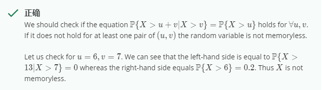
Week 2.5: Memoryless property
[Def] Memoryless Property:
A random variable $X$ possesses the memoryless property, $iff$
$\mathcal{P}\{X>u+v\} = \mathcal{P}\{X>u\} \mathcal{P}\{X>v\}$
If $\mathcal{P}\{x>v\}>0$, then
$\mathcal{P}\{ X>u+v \vert X>v \} = \mathcal{P}\{ X>u \}\ldots(\square)$
這是因為
$$\mathcal{P}\{X>u+v\} = \mathcal{P}\{X>u+v , X>v\}=\mathcal{P}\{X>u+v \vert X>v\}\mathcal{P}\{X>v\} \\
\text{mem.less prop.}\Rightarrow \mathcal{P}\{X>u\} \mathcal{P}\{X>v\} = \mathcal{P}\{X>u+v \vert X>v\}\mathcal{P}\{X>v\} \\
\Rightarrow \mathcal{P}\{X>u\} = \mathcal{P}\{X>u+v \vert X>v\}$$
從這就可以看出為何稱 memoryless. 這是因為 已經等了 $v$ 的時間, 要再多等 $u$ 的時間, 跟一開始就等 $u$ 的時間的機率是一樣的
再來有一個定理可以看出 Poisson process 適不適合用來 model 一個問題
[Thm] Memoryless is exactly exponential distribution:
Let $X$ be a random variable with density $p(x)$, 則
$X\text{ memoryless } \Longleftrightarrow p(x)=\lambda e^{-\lambda x}\text{, }X\sim\text{ exponential p.d.f.}$
範例: 公車每 $20 \pm 2$ 分鐘來一班, 也就是說 $X$ 是公車到的時間的 r.v. 值在 $20 \pm 2$. 這個問題是否可以用 Poisson process 來 model ? (檢察 r.v. $X$ 是否具有 memoryless property)
令 $v=19$, $u=10$, 則考慮 $(\square)$
L.H.S. 為 $\mathcal{P}\{X>29|X>19\}=0$
R.H.S. 為 $\mathcal{P}\{ X>10 \}=1$
兩者不相等, 所以不具有 memoryless property, 因此此 random variable 不能用在 renewal process 讓它成為 Poisson process
[Quiz]: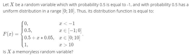
Week 2.6-7: Other definitions of Poisson processes
之前定義 Poisson process 是 renewal process 的一個特例 (當 $\xi$ 是 exponential distribution)
現在給出另一種定義, 這種定義跟 Poisson process 與 Levy precess 的關聯有很大的關係. (之後才會知道)
[Poisson Processes Def2] from Levy precess:
Poisson process is an integer-valued process, $N_t$, with $N_0=0$ a.s. (almost surely), such that
1. $N_t$ has independent increments
$\forall t_0<t_1<...<t_n$, we have $N_{t_1}-N_{t_0}, ..., N_{t_n}-N_{t_{n-1}}$ are independent
2. $N_t$ has stationary increments
$N_t-N_s$ 與 $N_{t-s}$ 具有相同的 distribution
3. $N_t-N_s\sim Pois(\lambda(t-s))$
$${\color{orange}
{
\mathcal{P}\{N_t=n\} \sim Pois(\lambda t)=e^{-\lambda t}\frac{(\lambda t)^n}{n!}
}
}$$
特性 3 可以推導出特性 2
$X \sim Pois(\mu)$ has $\mathbb{E}[X]=Var[X]=\mu$
我們再來推導一個定理, 該定理讓我們有第三種 Poisson process 的定義. 且跟 queueing theory 有關聯.
當在一個極短的時間段之內, Poisson process 能分成三種情況:
1. 沒有事件發生
2. 事件發生 $1$ 次
3. 事件發生 $\geq 2$ 次
定義 $f(h)=o(g(h))$ 為
$\lim_{h\rightarrow0}\frac{f(h)}{g(h)}=0$
直觀理解為 $f(h)$ 比 $g(h)$ 小的更快.
[Thm] Poisson process 在極小時間段的行為:
$$\left\{
\begin{array}{rl}
\mathcal{P}\{N_{t+h}-N_t=0\} = 1 -\lambda h + o(h), & h\rightarrow0 \\
\mathcal{P}\{N_{t+h}-N_t=1\} = \lambda h + o(h), & h\rightarrow0 \\
\mathcal{P}\{N_{t+h}-N_t\geq2\} = o(h), & h\rightarrow0
\end{array}
\right.$$
[Proof]:
我們先證明 $=0$ 的情況
根據之前的 定義2 我們知道 $\mathcal{P}\{N_{t+h}-N_t=0\}=e^{-\lambda h}$, 則
$$\lim_{h\rightarrow0}\frac{1-\mathcal{P}\{N_{t+h}-N_t=0\}}{h} = \lim_{h\rightarrow0}\frac{1-e^{-\lambda h}}{h}\\
\text{by L'Hospital's rule} = \lim_{h\rightarrow0}\frac{\lambda e^{-\lambda h}}{1} = \lambda$$
i.e., as $h\rightarrow0$,
$$\frac{1-\mathcal{P}\{N_{t+h}-N_t=0\}}{h} = \lambda + o(1) \\
\Rightarrow \mathcal{P}\{N_{t+h}-N_t=0\} = 1-\lambda h + ho(1) \\
= 1-\lambda h + o(h)$$
$o(h)$ 的正負號不重要, Q.E.D.
而 $\mathcal{P}\{N_{t+h}-N_t=1\} = \lambda h + o(h), h\rightarrow0$ 這一條可以藉由計算
$$\lim_{h\rightarrow0}\frac{\mathcal{P}\{N_{t+h}-N_t=1\}}{h} = \lim_{h\rightarrow0}\frac{e^{-\lambda h}\lambda h}{h}\\
\text{by L'Hospital's rule} = \lim_{h\rightarrow0}\frac{-\lambda e^{-\lambda h}\lambda h + \lambda e^{-\lambda h}}{1} = \lambda$$
i.e., as $h\rightarrow0$,
$$\frac{\mathcal{P}\{N_{t+h}-N_t=1\}}{h} = \lambda + o(1) \\
\Rightarrow \mathcal{P}\{N_{t+h}-N_t=1\} = \lambda h + o(h)$$
Q.E.D.
最後, $\mathcal{P}\{N_{t+h}-N_t\geq2\}=1-\mathcal{P}\{N_{t+h}-N_t=0\} - \mathcal{P}\{N_{t+h}-N_t=1\}$ 可以計算得到
注意到 $-o(h)=o(h)$, $2o(h)=o(h)$
Q.E.D.
[Poisson Processes Def3] from queueing process:
Poisson process is an integer-valued process, $N_t$, with $N_0=0$ a.s. (almost surely), such that
1. $N_t$ has independent increments
$\forall t_0<t_1<...<t_n$, we have $N_{t_1}-N_{t_0}, ..., N_{t_n}-N_{t_{n-1}}$ are independent
2. $N_t$ has stationary increments
$N_t-N_s$ 與 $N_{t-s}$ 具有相同的 distribution
3. 滿足:
$\lim_{h\rightarrow0} \frac{\mathcal{P}\{N_{t+h} - N_t\geq2\}}{\mathcal{P}\{N_{t+h}-N_t=1\}}=0$
定義 2 和定義 3 的差別只在第 3 點的條件. 然而兩種定義等價.
我們其實已經證明了 (定義 2 $\Rightarrow$ 定義 3), 但另一個方向還沒有
Week 2.8-9: Non-homogeneous Poisson processes
也可以參考 https://www.randomservices.org/random/poisson/Nonhomogeneous.html, 但對我來說有點難懂
[Non-homogeneous Poisson Processes Def1]:
Let $\Lambda(t)$ be a differentiable increasing function, and $\Lambda(0)=0$,
$N_t$ is a N.H.P.P. (Non-Homogeneous Poisson Processes), if
1. $N_0=0$
2. $N_t$ has independent increments
3. $N_t-N_s \sim Pois(\Lambda(t)-\Lambda(s))$
$${\color{orange}
{
\mathcal{P}\{N_t=n\} \sim Pois(\Lambda(t))=e^{-\Lambda(t)}\frac{\Lambda(t)^n}{n!}
}
}$$
定義 $\lambda(t) = \Lambda’(t)$, 稱 intensity function
在 P.P. 的定義 2, 我們知道 $N_t-N_s\sim Pois(\lambda(t-s))$, 所以當 $\Lambda(t)=\lambda t$ 的話, non-homogeneous P.P. 等於 P.P.
我們可以發現 non-homogeneous 去掉 stationary increment 特性, 也就是 Poisson distribution 的 rate $\lambda$ 在每個時間段落不一定會都一樣, depends on $\Lambda(t)$
[Properties of N.H.P.P.]:
1. $\mathbb{E}[N_t]=\Lambda(t)$
我們算一下 $\mathbb{E}[N_t]$ for N.H.P.P.:
$N_t = N_t - N_0 \sim Pois(\Lambda(t)-\Lambda(0))=Pois(\Lambda(t))$
$\therefore \mathbb{E}[N_t]=\Lambda(t)$
2. 如果 $\lambda(t)=\text{const} \Rightarrow \Lambda(t) = \text{const}\cdot t$, 回退到原來的 (homogeneous) P.P.
3. 因為 $\Lambda(t)$ is differentialble and increasing, 所以 $\Lambda^{-1}(t)$ 存在
讓我們假設 $\text{Image}(\Lambda(t))=\mathbb{R}^+$, 所以 $\Lambda^{-1}(t)$ 對於 $t\in\mathbb{R}^+$ 都是 well defined
對於一個 N.H.P.P. 的 $N_t$ 來說, 考慮 $N_{\Lambda^{-1}(t)}$ 這些 r.v.s 的話, 會發現變成了 homogeneous P.P. 了!
第三點提供了一個 N.H.P.P. 與 P.P. 的對應方法
但具體來說, 如果一個 N.H.P.P. 剛好是 P.P. 的話, iff 他也是個 renewal process, 下一節證明
Week 2.10-12: Relation between renewal theory and non-homogeneous Poisson processes
我們試著從一個 $N_t$ 是 N.H.P.P. 去建構 renewal process 看看, 我們有如下的 N.H.P.P.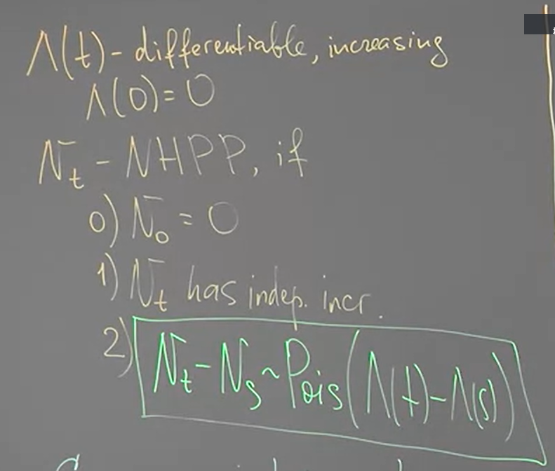
Renewal process 的 arrival time $S_n$ 可以這麼構建
$S_n=\arg\min_t\{N_t=n\}$
有 $S_n$ 就可以得到 interarrival time $\xi_n=S_n-S_{n-1}$
這樣子的 arrival times $S_n$ and interarrival times $\xi_n$ 是一個 renewal process 嗎?
首先我們知道若要成為一個 renewal process, $\xi_1, \xi_2, …$ 必須是 i.i.d. 才行
Note that:
$${
\mathcal{P}\{N_t=n\} \sim Pois(\Lambda(t))=e^{-\Lambda(t)}\frac{\Lambda(t)^n}{n!}
}$$
先證明以下兩個等式:
$\mathcal{P}_{\xi_1}(x)=\lambda(x)e^{-\Lambda(x)}$:
[Proof]:
$$\mathcal{P}\{\xi_1\leq x\}=\mathcal{P}\{S_1\leq x\}=\mathcal{P}\{N_x\geq 1\} = 1 - \mathcal{P}\{N_x=0\} \\ = 1- Pois(\Lambda(x)) = 1-e^{-\Lambda(x)}$$
用到 $\{S_n\leq t\}=\{N_t\geq n\}$, 然後左右等式微分得到:
$\mathcal{P}_{\xi_1}(x)=\lambda(x)e^{-\Lambda(x)}$
其中 $\lambda=\Lambda’$, Q.E.D.- $\mathcal{P}_{(\xi_2|\xi_1)}(t|s)=\lambda(t+s)e^{-\Lambda(t+s)+\Lambda(s)}$:
[Proof]:
先計算一下兩個 r.v.s $\xi_1,\xi_2$ 的 joint C.D.F. $\mathcal{F}_{\xi_1,\xi_2}(s,t)$$$\mathcal{F}_{(\xi_1,\xi_2)}(\xi_1=s,\xi_2=t)=\mathcal{P}\{\xi_1\leq s, \xi_2\leq t\} \\ =\int_{y=0}^s \mathcal{P}\{ \xi_1\leq s, \xi_2\leq t \vert \xi_1=y \} \mathcal{P}_{\xi_1}(y)dy$$
$\because y\leq s$
$$=\int_{y=0}^s \mathcal{P}\{ \xi_2\leq t \vert \xi_1=y \} \mathcal{P}_{\xi_1}(y) dy \\ = \int_{y=0}^s \mathcal{P}\{ N_{t+y} - N_y \geq 1 \vert \xi_1 = y \} \mathcal{P}_{\xi_1}(y) dy \ldots(\star)$$
由 N.H.P.P. 的 independent increments 特性知道 $(N_{t+y} - N_y),(N_y-N_0)$ 這兩個 r.v.s 為 independent. 因此
$$\mathcal{P}\{N_{t+y} - N_y \geq 1 | \xi_1=y\} = \mathcal{P}\{ N_{t+y} - N_y \geq 1 | N_y-N_0=1 \} \\ = \mathcal{P}\{N_{t+y} - N_y \geq 1 \}$$
接續 $(\star)$
$$(\star) = \int_{y=0}^s \mathcal{P}\{ N_{t+y}-N_y \geq 1 \} \cdot \mathcal{P}_{\xi_1}(y) dy \\ = \int_{y=0}^s (1 - \mathcal{P}\{ N_{t+y}-N_y = 0 \}) \cdot \mathcal{P}_{\xi_1}(y) dy \\ = \int_{y=0}^s (1 - e^{-\Lambda(t+y)+\Lambda(y)}) \cdot \lambda(y)e^{-\Lambda(y)} dy$$
所以兩個 r.v.s $\xi_1,\xi_2$ 的 joint C.D.F.
$\mathcal{F}_{(\xi_1,\xi_2)}(s,t) = \int_{y=0}^s (1 - e^{-\Lambda(t+y)+\Lambda(y)}) \cdot \lambda(y)e^{-\Lambda(y)} dy$
微分可以計算 P.D.F.
$$\mathcal{P}_{(\xi_1,\xi_2)}(s,t) = \frac{\partial}{\partial t} \left( \frac{\partial}{\partial s} \mathcal{F}_{(\xi_1,\xi_2)}(s,t) \right) \\ \text{replace y by s} = \frac{\partial}{\partial t} \left( (1 - e^{-\Lambda(t+s)+\Lambda(s)}) \cdot \lambda(s)e^{-\Lambda(s)} \right) \\ = \lambda(t+s) e^{-\Lambda(t+s)+\Lambda(s)}\cdot \lambda(s) e^{-\Lambda(s)} \\ = \lambda(t+s) e^{-\Lambda(t+s)+\Lambda(s)} \cdot \mathcal{P}_{\xi_1}(s)$$
所以
$$\mathcal{P}_{(\xi_2|\xi_1)}(t|s) = \frac{\mathcal{P}_{(\xi_1,\xi_2)}(s,t)}{\mathcal{P}_{\xi_1}(s)} \\ =\lambda(t+s)e^{-\Lambda(t+s)+\Lambda(s)}$$
Q.E.D.
回到考慮什麼情況下的 N.H.P.P. 的 $\xi_1, \xi_2, …$ 是 i.i.d. 這個問題
我們先假設 $\xi_1, \xi_2, …$ 是 i.i.d., i.e. 假設 N.H.P.P. 是 renewal process, 則
$$\mathcal{P}_{\xi_2 | \xi_1}(t|s)=\mathcal{P}_{\xi_2}(t) \\
\because\text{i.i.d.}=\mathcal{P}_{\xi_1}(t), \forall t,s>0$$
帶入我們花很多力氣推導的上述兩個結果得到:
$\lambda(t+s)e^{-\Lambda(t+s)+\Lambda(s)} = \lambda(t)e^{-\Lambda(t)}$
然後對兩邊都做積分
$(\square)$ R.H.S.:
$$\int_0^T \lambda(t)e^{-\Lambda(t)} dt = \int_0^T e^{-\Lambda(t)}d\Lambda(t) \left(= \int_0^Te^{-y}dy\right) \\
= -e^{-\Lambda(T)}+e^{-\Lambda(0)} = 1 -e^{-\Lambda(T)}$$
$(\square)$ L.H.S. 同理
$$\int_0^T\lambda(t+s)e^{-\Lambda(t+s)+\Lambda(s)} dt = e^{\Lambda(s)}\int_0^T e^{-\Lambda(t+s)} d\Lambda(t+s) \\
\left(\text{this as: }e^{\Lambda(s)}\int e^{-y}dy\right) \\
= e^{\Lambda(s)}
\left[\left.
-e^{\Lambda(t+s)}\right|_{t=0}^T
\right] = e^{\Lambda(s)}\left[-e^{-\Lambda(T+s)}+e^{-\Lambda(s)}\right] = -e^{-\Lambda(T+s)+\Lambda(s)}+e^0$$
所以 L.H.S = R.H.S.
$$\Rightarrow e^0-e^{-\Lambda(T+s)+\Lambda(s)} = 1 - e^{-\Lambda(T)} \\
\Rightarrow \Lambda(T+s) - \Lambda(s) = \Lambda(T), \forall T,s>0$$
因為 $\Lambda$ is increasing function, 上式知道是 linear function, 所以會得到 $\Lambda(t)=\text{const}\cdot t$
而這正好表明了 N.H.P.P. 變成了 homogeneous P.P. 了
結論是:
N.H.P.P. is a renewal process $\Longleftrightarrow$ $\Lambda (t)=\lambda t$ (i.e. 此時的 N.H.P.P. 也變成 homogenous 了)
$(\Longleftarrow)$ 證明很容易, 因為 homogeneous P.P. 是 renewal process
換句話說 N.H.P.P. is a renewal process $\Longleftrightarrow$ it is homogenous P.P.
Week 2.13: Elements of the queueing theory. M/G/k systems-1
我們先前證明過
[Thm] Poisson process 在極小時間段:
$$\left\{
\begin{array}{rl}
\mathcal{P}\{N_{t+h}-N_t=0\} = 1 -\lambda h + o(h), & h\rightarrow0 \\
\mathcal{P}\{N_{t+h}-N_t=1\} = \lambda h + o(h), & h\rightarrow0 \\
\mathcal{P}\{N_{t+h}-N_t\geq2\} = o(h), & h\rightarrow0
\end{array}
\right.$$
對於 N.H.P.P. 也有類似的結果
[Thm] Non-homogeneous Poisson process 在極小時間段:
$$\left\{
\begin{array}{rl}
\mathcal{P}\{N_{t+h}-N_t=0\} = 1 -{\color{orange}{\lambda(t)}} h + o(h), & h\rightarrow0 \\
\mathcal{P}\{N_{t+h}-N_t=1\} = {\color{orange}\lambda(t)} h + o(h), & h\rightarrow0 \\
\mathcal{P}\{N_{t+h}-N_t\geq2\} = o(h), & h\rightarrow0
\end{array}
\right.$$
所以類似的對於 N.H.P.P. 我們也有另一種定義 (類似 [Poisson Processes Def3])
[Non-homogeneous Poisson Processes Def2]:
Let $\Lambda(t)$ be a differentiable increasing function, and $\Lambda(0)=0$,
$N_t$ is a N.H.P.P. (Non-Homogeneous Poisson Processes), if
1. $N_0=0$
2. $N_t$ has independent increments
3. 滿足:
$\lim_{h\rightarrow0} \frac{\mathcal{P}\{N_{t+h} - N_t\geq2\}}{\mathcal{P}\{N_{t+h}-N_t=1\}}=0$
(Non-homogeneous) Poisson processes 很適合用來 modeling queueing processes.
我們用 $M,D,G$ 來表示 distribution 種類:
- $M$: exponential distribution. 所以如果用來描述 arrival processes (memoryless) 就會變成 Poisson processes
- $D$: deterministic (constant distribution, 即不受 time $t$ 的影響? 還是連 value 都是 constant?)
- $G$: general, 表示可以是任何 distribution
Queueing processes 包含了三個字母, e.g. $M/G/k$, 分別表示 Arrival process, Service time, 和 Number of servers
- Arrival process: $\in\{M,D,G\}$
- Service time: $\in\{M,D,G\}$. 同時為 I.I.D.
- Number of servers: $\in\{1, 2, ..., \infty\}$
我們以學生上機房用電腦來舉例, 若用 queueing process 為 $M/G/\infty$ 來描述的話
Arrival processes (by Poisson process) 描述了學生來的 $N(t)$
Service time 表示學生會用多久電腦, 用 $G_Y(t)$ 這個 distribution 描述
而電腦 (server) 的數量為 $\infty$, 表示學生一到就馬上有一台電腦可以用, 無需等待 (更複雜的 queueing process 會考慮等待時間)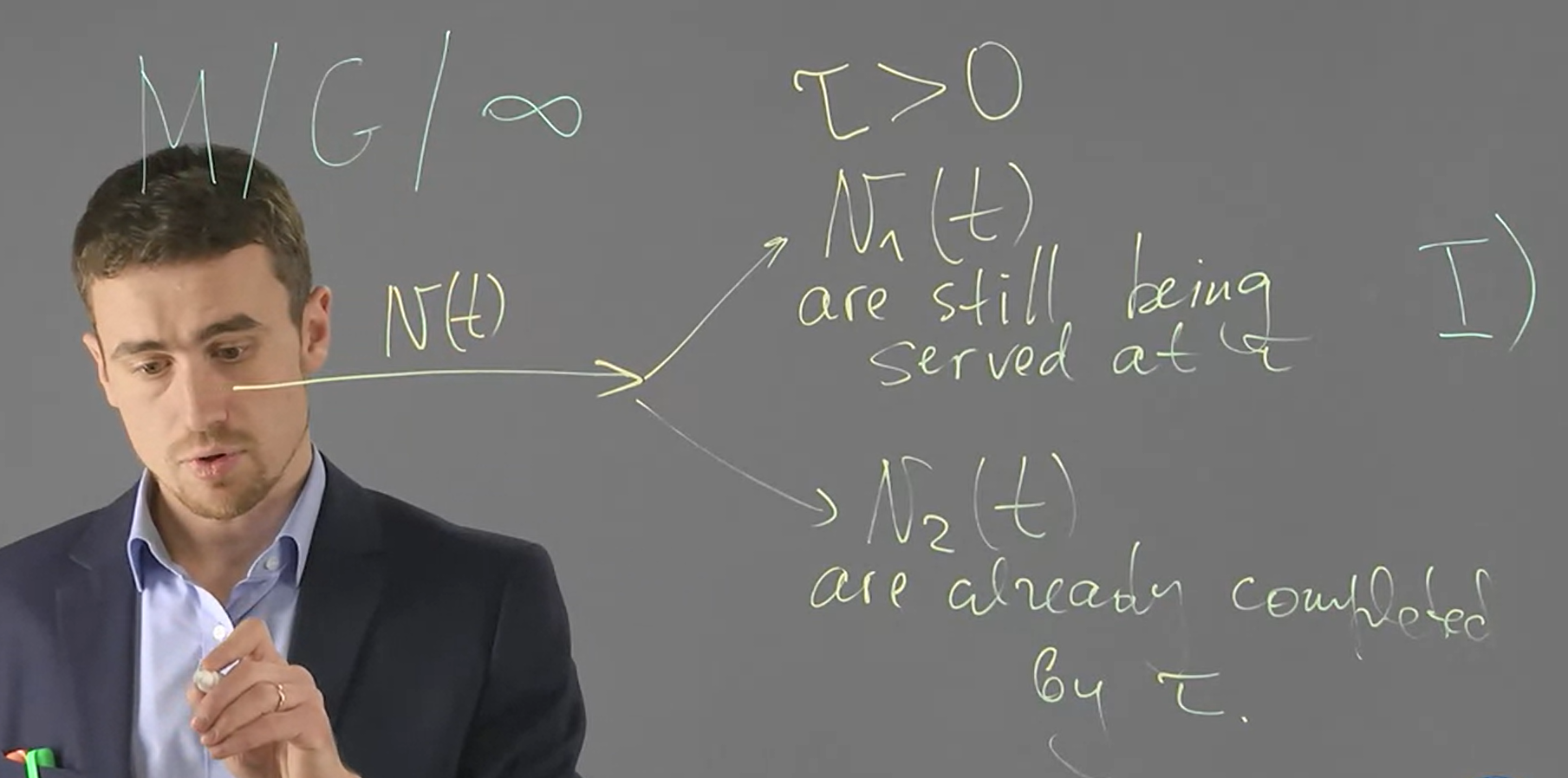
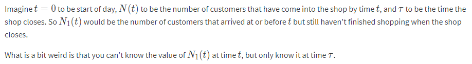
所以 $N(t)$ 是一個 Poisson process, 考慮一個 fixed time $\tau>0$, 我們會有兩個 processes $N_1(t)$ and $N_2(t)$.
$N_1(t)$ 表示有多少 還在處理 的事件 at time $\tau$ (即在時間 $\tau$ 還有多少學生在用電腦)
$N_2(t)$ 表示有多少 已處理完 的事件 at time $\tau$ (即在時間 $\tau$ 已有多少學生用完電腦)
$t$ and $\tau$ 的關係在討論區有人這麼回答
考慮 $N_1(t+h) - N_1(t)$, 這個值表示在這一段時間內共來了多少事件並且還在處理 (即這段時間來了多少學生, 並且這些學生都還在用電腦), 所以:
$$\mathcal{P}\{ N_1(t+h)-N_1(t)=1 \} \\
= \mathcal{P}\{ N(t+h)-N(t)=1 \} \cdot \mathcal{P}\{ Y>\tau-t \} + o(h) \ldots(\blacktriangle)$$
$Y$ 表示 service time 的 random variable, 其 distribution 為 $G_Y(t)$
“這段 $h$ 時間來了多少學生, 並且這些學生都還在用電腦” 可以近似於:
“這段 $h$ 時間來了 $1$ 個學生, 並且這 $1$ 個學生還在用電腦” + $o(h)$
注意到 $2$ 個學生以上的情形我們用 $o(h)$ 表示即可, 這是因為 Poisson process 的一個性質:
$\mathcal{P}\{N_{t+h}-N_t\geq2\} = o(h),h\rightarrow0$
所以用上開頭的 Theorem,
$$(\blacktriangle) = (\lambda h + o(h)) \cdot (1-G_Y(\tau-t)) + o(h) \\
= \lambda h(1-G_Y(\tau-t)) + o(h)$$
重述一遍, 我們有:
$\mathcal{P}\{ N_1(t+h)-N_1(t)=1 \} = \lambda(1-G_Y(\tau-t))h + o(\delta)$
令 $\lambda(1-G_Y(\tau-t))$ 等於某個 function $\lambda_1(t)$, 則上式與 N.H.P.P. 的性質結果相同.
同樣可以對 $\mathcal{P}\{ N_1(t+h)-N_1(t)=0 \}$ 和 $\mathcal{P}\{ N_1(t+h)-N_1(t)\geq2 \}$ 推導出相同結果.
所以根據 [Non-homogeneous Poisson Processes Def2] 我們得到 $N_1$ 是 N.H.P.P. 的結論
$N_1$ 是 N.H.P.P. 且其 intensity function $\lambda_1(t)=\lambda(1-G_Y(\tau-t))$
我們對於 $N_1$ 的推論同樣也可以用在 $N_2$ 上, 結果也是一樣:
$N_2$ 是 N.H.P.P. 且其 intensity function $\lambda_2(t)=\lambda \cdot G_Y(\tau-t)$
下一節課會證明 $N_1$ and $N_2$ 為互相獨立的 r.v.s
Week 2.14: Elements of the queueing theory. M/G/k systems-2
欲證 $\mathcal{P}\{N_1(t)=n_1, N_2(t)=n_2\} = \mathcal{P}\{N_1(t)=n_1\}\mathcal{P}\{ N_2(t)=n_2\}$
$$\mathcal{P}\{N_1(t)=n_1, N_2(t)=n_2\}\\
= \mathcal{P}\{ N_1(t)=n_1, N_2(t)=n_2 | N(t)=n_1+n_2 \} \cdot \mathcal{P}\{N(t)=n_1+n_2\} \\
= \mathcal{C}_{n_1}^{n_1+n_2}(1-G(\tau-t))^{n_1}(G(\tau-t))^{n_2} \cdot e^{-\lambda t}\frac{(\lambda t)^{n_1+n_2}}{(n_1+n_2)!} \ldots(=)$$
$(=)$ 為 Binomial term, 把”成功”的機率當成 “事件在時間 $\tau$ 還在served的機率”, 這個機率由 service time 的 distribution probability 可以知道:
$\mathcal{P}\{Y>(\tau-t)\}=1-\mathcal{P}\{Y\leq(\tau-t)\}=1-G(\tau-t)$
所以失敗的話就是 $G(\tau-t)$
共有 $n$ 個事件, 共有 $n_1$ 個事件 $\in N_1(t)$, and $n_2$ 個事件 $\in N_2(t)$, 所以 $\mathcal{C}_{n_1}^{n_1+n_2}$
我不知道的是為何 $\frac {(\lambda t(1-G(\tau-t)))^{n_1}}{n_1!} e^{-\lambda t(1-G(\tau-t))} = \mathcal{P}\{N_1(t)=n_1\}$
因為只知道 $N_1$ 是 N.H.P.P. 且其 intensity function $\lambda_1(t)=\lambda(1-G_Y(\tau-t))$
所以必須求得 $\Lambda_1(t)$ 才能代入
$\mathcal{P}\{N_t=n\} \sim Pois(\Lambda(t))=e^{-\Lambda(t)}\frac{\Lambda(t)^n}{n!}$
所以看起來 $\Lambda_1(t)=\lambda t(1-G(\tau-t))?$ 不懂…
Q.E.D.
Week 2.15-17: Compound Poisson processes
可參考一個淺顯易懂的定義: https://gtribello.github.io/mathNET/COMPOUND_POISSON_PROCESS.html
[Compound Poisson Processes (C.P.P.) Def]:
$X_t=\sum_{k=1}^{N_t} \xi_k$
其中
- $N_t$ 是 Poisson process with intensity $\lambda$
- $\xi_1,\xi_2,…$ are i.i.d.
- $\xi_1,\xi_2,…$ and $N_t$ are independent
$X_t$ 的 distribution 沒有 cloded form, 但若是某些特定的 $\xi$ distribution 可以算出來.
注意到若 $\xi_k=1$, 則 $X_t=N_t$, 可藉此想像一下 C.P.P. 的物理意義
如果 $\xi$ (C.P.P.) 是 non-negative integer values, 我們使用 PGF 幫助計算
[Probability Generating Function (PGF) Def]:
Let $\xi$ 是一個 integer 的 random variable, with $\geq 0$ values. 則 PGF 定義為:
$\varphi_\xi(u)=\mathbb{E}[u^\xi], \text{ where }|u|<1$
根據定義我們可以得到 (expectation 寫出來), 如果 $\xi_1 \perp \xi_2$, 則 $\varphi_{\xi_1+\xi_2}(u)=\varphi_{\xi_1}(u)\varphi_{\xi_2}(u)$
如果 $\xi$ (C.P.P.) 是 non-negative (real) values, 我們使用 MGF 幫助計算
[Moment Generating Function (MGF) Def]:
跟 Laplace transform 密切相關.
$\mathcal{L}_\xi(u)=\mathbb{E}[e^{-u\xi}], \text{ where } \xi\geq0, u>0$
其實就是 $\mathcal{L}_f(s)=\int_{x=0}^\infty e^{-sx}f(x)dx$, 將 $f$ 以 $\xi$ 的 P.D.F. 代入
根據定義我們可以得到, 如果 $\xi_1 \perp \xi_2$, 則 $\mathcal{L}_{\xi_1+\xi_2}(u)=\mathcal{L}_{\xi_1}(u)\mathcal{L}_{\xi_2}(u)$. 注意到 ${\xi_1+\xi_2}$ 其 P.D.F. 是 $\xi_1,\xi_2$ 的 P.D.F.s 的 convolution. 之前我們也證過 Laplace transform 這個性質
對於 $\xi$ (C.P.P.) 是 general case 的情況來說, 我們需借助 characteristic function 幫忙
[Characteristic Function Def]:
For random variable $\xi$, 定義 characteristic function $\Phi:\mathbb{R}\rightarrow \mathbb{C}$ 為
$\Phi_\xi(u) = \mathbb{E}\left[ e^{iu\xi} \right]$
同樣根據定義我們可以得到, 如果 $\xi_1 \perp \xi_2$, 則 $\Phi_{\xi_1+\xi_2}(u)=\Phi_{\xi_1}(u)\Phi_{\xi_2}(u)$
[Characteristic Function of Increment of C.P.P.]:
For $t>s\geq0$, and $X_t$ is a C.P.P., we have
$\Phi_{X_t-X_s}(u)=e^{\lambda(t-s)(\Phi_{\xi_1}(u)-1)}$
[Proof]:
$$\Phi_{X_t-X_s}(u)=\mathbb{E}\left[ e^{iu(X_t-X_s)} \right] \\
=\sum_{k=0}^\infty
{\color{orange}
{\mathbb{E}\left[ \left. e^{iu(X_t-X_s)} \right| N_t-N_s=k\right]}
}
\cdot
{\color{green}
{\mathcal{P}\{N_t-N_s=k\}}
}$$
注意到已知 $N_t-N_s=k$ 的情況下, $X_t-X_s$ 根據 C.P.P. 的定義就是 $\xi_1+…+\xi_k$, 再加上我們知道 $\xi\perp N_t$, 所以橘色部分的 condition 就可以拔掉. 同時已知綠色部分為 Poisson Processes.
因此:
$$= \sum_{k=0}^\infty
\mathbb{E}\left[e^{iu(X_t-X_s)}\right] \cdot
Pois(\lambda(t-s)) \\
= \sum_{k=0}^\infty
(\Phi_{\xi_1}(u))^k \cdot e^{-\lambda(t-s)}\frac{(\lambda(t-s))^k}{k!} \\
=e^{-\lambda(t-s)}\sum_{k=0}^\infty\frac{(\Phi_{\xi_1}(u)\lambda(t-s))^k}{k!} \\
= e^{-\lambda(t-s)}e^{\Phi_{\xi_1}(u)\lambda(t-s)} =e^{\lambda(t-s)(\Phi_{\xi_1}(u)-1)}$$
Q.E.D.
此定理描述了 increment of C.P.P. 的 characteristic function, 其具有 closed form solution
所以 characteristic function of $X_t$ is
$\Phi_{X_t}(u)=e^{\lambda t(\Phi_{\xi_1}(u)-1)}$
課程老師說這個 Theorem 很重要, 可以根據它推導出很多 Corollaries
[Expectation and Variance of C.P.P.]:
對於此節定義的 C.P.P. 我們有
$$\mathbb{E}[X_t]=\lambda t\mathbb{E}[\xi_1] \\
Var[X_t]=\lambda t\mathbb{E}[\xi_1^2]$$
原來的 Poisson distribution $Pois(\lambda t)$ 的 mean and variance 為 $\lambda t$, 所以 C.P.P. 等於多乘上 $\xi_1$ 的 moments
[Proof]:
課程證 expectation, 而 variance 可用同樣流程證明
$\mathbb{E}[\xi^r]<\infty\Rightarrow\Phi_\xi(u)$ is r-times 可微 at 0
因為 derivative and expectation 都是線性的, 所以我們有
$\Phi^{(1)}_\xi(u)=\frac{d}{du}\mathbb{E}[e^{iu\xi}]=\mathbb{E}[(i\xi)e^{iu\xi}]$
$\Phi^{(2)}_\xi(u)=\frac{d}{du}\frac{d}{du}\mathbb{E}[e^{iu\xi}]=\mathbb{E}[(i\xi)^2 e^{iu\xi}]$
$…$
$\Phi^{(r)}_\xi(u)=\mathbb{E}[(i\xi)^r e^{iu\xi}]$
$\therefore \Phi_\xi^{(r)}(0)=i^r\cdot\mathbb{E}[\xi^r]$
由前面的 Theorem 知道 $\Phi_{X_t}(u)=e^{\lambda t(\Phi_{\xi_1}(u)-1)}$, 所以
$$\Phi_{X_t}^{(1)}(u)=\frac{d}{du}\Phi_{X_t}(u) =\frac{d}{du}e^{\lambda t(\Phi_{\xi_1}(u)-1)} \\
=\lambda t \Phi_{\xi_1}^{(1)}(u)e^{\lambda t(\Phi_{\xi_1}(u)-1)} = \lambda t \Phi_{\xi_1}^{(1)}(u)\Phi_{X_t}(u)$$
計算 $\mathbb{E}[X_t]$:
$$\mathbb{E}[X_t]=\frac{\Phi_{X_t}^{(1)}(0)}{i}
= \frac{\lambda t \Phi_{
\xi_1}^{(1)}(0) \overbrace{\Phi_{X_t}(0)}^{=1}
}
{i}$$
而根據 characteristic function 的特性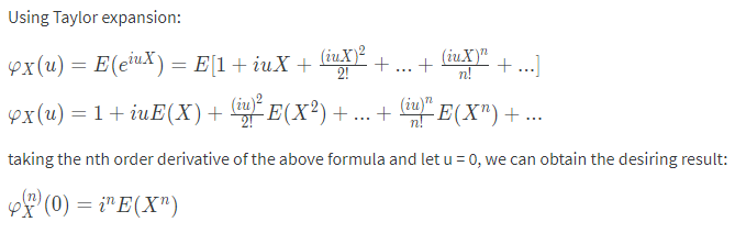
$\frac{\Phi_{\xi_1}^{(1)}(0)}{i} = \mathbb{E}[\xi_1]$
所以 $\mathbb{E}[X_t]=\lambda t\mathbb{E}[\xi_1]$
Q.E.D.
Applications of the Poisson Processes and Related Models
Applications of the Poisson Processes and Related Models.pdf