Stochastic Processes Week 4 Gaussian Processes

Coursera Stochastic Processes 課程筆記, 共十篇:

Week 4.1: Random vector. Definition and main properties

Normal distribution of one r.v.
$$X\sim\mathcal{N}(\mu,\sigma^2), \text{ for }\sigma>0,\mu\in\mathbb{R} \\ p(x)=\frac{1}{\sqrt{2\pi}\sigma} e^{-\frac{(x-\mu)^2}{2\sigma^2}}$$
The characteristic function of normal distribution is:
$\Phi(u)=e^{iu\mu-\frac{1}{2}u^2\sigma^2}$
我們可以說一個 random variable $X$ almost surely constant $=\mu$ 表示如下:
$\mathcal{P}\{X=\mu\}=1$
如果此時也定義 $\sigma=0$, 我們可將其也視為 normal distribution $\mathcal{N}(\mu,0)$

等於把 constant 也加入 normal distribution 的定義

[Gaussian Vector Def]:
A random vector $\vec{X}=(X_1,...,X_n)$ is Gaussian if and only if
$$(\star):\sum_{k=1}^n \lambda_k X_k \sim \mathcal{N}\\ \forall(\lambda_1,...,\lambda_n)\in\mathbb{R}$$

Week 4.2: Gaussian vector. Definition and main properties

Definition of multivariate characteristic function, ref from wiki

我們說明一下為何 $C$ (covariance matrix) is positive semi-definite, 檢查 $\vec{u}^TC\vec{u},\forall \vec{u}$
$$\vec{u}^TC\vec{u} = \sum_{k,j=1}^n u_k c_{kj} u_j = \sum_{k,j=1}^n u_k Cov(X_j,X_k) u_j \\ = Cov\left(\sum_{j=1}^n u_jX_j,\sum_{k=1}^n u_kX_k\right) = Var\left(\sum_{j=1}^n u_jX_j\right) \geq 0$$

[Gaussian Vector Thm]:
$\vec{X}$ is Gaussian vector if and only if any of the following conditions holds:
1. Characteristic function of Gaussian vector:
$$(\square): \Phi_{\vec{X}}(\vec{u})=\mathbb{E}\left[ e^{i\cdot \vec{u}^T\vec{X}} \right] = \exp\left\{ i\cdot \vec{u}^T\vec{\mu} - \frac{1}{2}\vec{u}^TC\vec{u} \right\} \\ \text{where }\vec{\mu}\in\mathbb{R}^n; C\in\mathbb{R}^{n\times n}\text{-positive semi-definite}$$
同時 $\vec{\mu}$ and $C$ 為
$$\vec{\mu}=(\mathbb{E}X_1,...,\mathbb{E}X_n) \\ C=\left(c_{jk}\right)_{j,k=1}^n; c_{jk}=Cov(X_j,X_k)$$
2. Can be represented by Standard Gaussian vector $\vec{X^o}$
$$(\blacksquare):\vec{X}=A\cdot \vec{X^o}+\vec{\mu} \\ \text{where }A\in\mathbb{R}^{n\times n},\vec{X^o}\text{ is standard Gaussin vector}$$
同時 $A=C^{1/2}$, i.e. $AA=C$

要寫出 $A$ 只要將 $C$ 對角化, 然後對中間的 diagonal matrix (eigenvalues 組成的) 取 sqrt 即可

[Proof]:
我們先證明 Definition $(\star)\Rightarrow 1.(\square)$
Let $\xi=\vec{u}^T\vec{X}=\sum_{k=1}^n u_kX_k$ 根據定義 $\xi\sim\mathcal{N}$
我們將 $\vec{X}$ 的特徵方程式寫出來:
$\Phi_{\vec{X}}(\vec{u})=\mathbb{E} [e^{i\vec{u}^T\vec{X}}]=\mathbb{E}[e^{i\xi\cdot1}]=\Phi_\xi(1)$
因為 $\xi\sim\mathcal{N}$, 所以特徵方程式是知道的:
$\Phi_\xi(1)=\exp\left(i\mu_\xi-\frac{1}{2}\sigma_\xi^2\right)$
所以我們只需計算出 $\mu_\xi,\sigma_\xi^2$ 在代回去即可
$\mu_\xi=\mathbb{E}\left[\sum_{k=1}^n u_kX_k\right] = \sum_{k=1}^n u_k \mu_k = \vec{u}^T \vec{\mu}$
$$\sigma_\xi^2 = cov\left( \sum_{k=1}^n u_k X_k, \sum_{j=1}^n u_j X_j \right) \\ = \sum_{k,j=1}^n u_k\cdot cov(X_k,X_j) \cdot u_j = \vec{u}^TC\vec{u}$$
代回去即可發現 $=(\square)$
Q.E.D.
我們再證明 $1.(\square)\Rightarrow$ Definition $(\star)$
因為特徵函數跟 P.D.F. 是一對一對應的, 所以知道 $\vec{X}$ 的特徵函數為 $(\square)$
很顯然這是 Gaussian 的特徵函數, 所以 $\vec{X}$ 是 Gaussian vector
證明 $2. (\blacksquare) \Rightarrow 1. (\square)$
$\vec{X}^o$ is standard Gaussian vector, 我們將它的特徵函數寫下來:
$\Phi_{\vec{X}^o}(\vec{u}) = \exp\{-\frac{1}{2}\vec{u}^T\vec{u}\}$
計算 $\vec{X}$ 的特徵函數:
$$\text{from }(\blacksquare) \text{ we know that } \Phi_{\vec{X}}(\vec{u})=\mathbb{E}\left[ e^{i\vec{u}^T(A\vec{X}^o+\vec{\mu})} \right] \\ = e^{i\vec{u}^T\vec{\mu}} \cdot \Phi_{\vec{X}^o}(A^T\vec{u}) \\ = e^{i\vec{u}^T\vec{\mu}} \cdot e^{-\frac{1}{2}\vec{u}^TAA^T\vec{u}} \\ = e^{i\vec{u}^T\vec{\mu}} \cdot e^{-\frac{1}{2}\vec{u}^TC\vec{u}} = (\square)$$
Q.E.D.
證明 $1. (\square) \Rightarrow 2. (\blacksquare)$
我們定義 $A:=C^{1/2}$, 則代入 $(\square)$ 再整理一下可以得到這是一個 $\vec{X}=A\cdot \vec{X^o}+\vec{\mu}$ 的特徵函數
Q.E.D.

Week 4.3: Connection between independence of normal random variables and absence of correlation

[Thm]:
Let $X_1,X_2\sim\mathcal{N}(0,1)$ and $corr(X_1,X_2)=0$, 則
$X_1 \perp X_2 \Longleftrightarrow (X_1,X_2) \text{ is Gaussian vector}$
[Proof]:
證明 $(\Rightarrow)$
$\lambda_1 X_1+\lambda_2 X_2 \sim \mathcal{N} \Longrightarrow (X_1,X_2) \text{ is Gaussian vector}$
可以從特徵方程式對於獨立 r.v.s 的線性組合, 以及 Gaussian 的特徵方程式看出來

證明 $(\Leftarrow)$
因為 uncorrelated
$$\therefore C=\left[ \begin{array}{c} 1 & 0 \\ 0 & 1 \end{array} \right] \Rightarrow A=\left[ \begin{array}{c} 1 & 0 \\ 0 & 1 \end{array} \right]=C^{1/2}$$
定理 $2. (\blacksquare)$ 告訴我們 $(X_1,X_2)$ 可以改寫如下:
$$\left[ \begin{array}{c} X_1 \\ X_2 \end{array} \right] =^d \left[ \begin{array}{c} 1 & 0 \\ 0 & 1 \end{array} \right] \left[ \begin{array}{c} \xi_1 \\ \xi_2 \end{array} \right] + \left[ \begin{array}{c} 0 \\ 0 \end{array} \right]$$
$=^d$ 表示相同分布, $\xi_1,\xi_2\sim\mathcal{N}(0,1)$
乘開來就發現 $X_1 =^d \xi_1$ and $X_2 =^d \xi_2$, 因此 $X_1 \perp X_2$
Q.E.D.

[Exercise1]:
Given $X_1\sim\mathcal{N}(0,1)$, $\mathcal{P}\{\xi=1\}=0.5; \mathcal{P}\{\xi=-1\}=0.5$,
and $\xi\perp X_1$
考慮 $X_2 = |X_1|\cdot \xi$, 證明 $X_2 \sim \mathcal{N}(0,1)$
[Proof]:
$$\mathcal{P}\{X_2\leq x\},\forall x>0\\ = \mathcal{P}\{|X_1|\leq x | \xi=1\}\mathcal{P}\{\xi=1\} + \mathcal{P}\{|X_1|\geq -x | \xi=-1\}\mathcal{P}\{\xi=-1\} \\ \text{Note }(X_1\perp\xi\text){ }= \mathcal{P}\{|X_1|\leq x\}/2 + \mathcal{P}\{|X_1|\geq -x\}/2 \\ \text{Note }(\mathcal{P}\{|X_1|\geq-x\}=1) = \frac{1}{2}\left( 1+\mathcal{P}\{|X_1|\leq x\} \right)\\ \text{by std normal} = \mathcal{P}\{X_1\leq x\}$$
注意到 Standard normal $\mathcal{P}\{X_1\geq x\}=\mathcal{P}\{X_1\leq -x\}$, 所以
$$\frac{1}{2}\left( 1+\mathcal{P}\{|X_1|\leq x\}\right) = \frac{1}{2}\left( 1 +\mathcal{P}\{X_1\leq x\}-\mathcal{P}\{X_1\leq -x\}\right) \\ = \frac{1}{2}\left( {\color{orange}1} +\mathcal{P}\{X_1\leq x\}-\mathcal{P}\{X_1\geq x\}\right) \\ = \frac{1}{2}\left( \color{orange}{\mathcal{P}\{X_1\leq x\}+\mathcal{P}\{X_1\geq x\}} +\mathcal{P}\{X_1\leq x\}-\mathcal{P}\{X_1\geq x\}\right) \\ = \mathcal{P}\{X_1\leq x\}$$
Q.E.D.

[Exercise2]:
Given $X_1\sim\mathcal{N}(0,1)$, $\mathcal{P}\{\xi=1\}=0.5; \mathcal{P}\{\xi=-1\}=0.5$, and $\xi\perp X_1$
考慮 $X_2 = |X_1|\cdot \xi$, 證明 $cov(X_1,X_2)=0$
[Proof]:
$$cov(X_1,X_2)=\mathbb{E}[X_1X_2]-\mathbb{E}[X_1]\mathbb{E}[X_2] \\ =\mathbb{E}[X_1\cdot|X_1|\cdot\xi]-0\cdot \mathbb{E}[X_2] \\ =\mathbb{E}[X_1\cdot|X_1|] \mathbb{E}[\xi] = \mathbb{E}[X_1\cdot|X_1|]\cdot 0=0$$
Q.E.D.

[Exercise3]:
Given $X_1\sim\mathcal{N}(0,1)$, $\mathcal{P}\{\xi=1\}=0.5; \mathcal{P}\{\xi=-1\}=0.5$, and $\xi\perp X_1$
考慮 $X_2 = |X_1|\cdot \xi$, 證明 $X_1$ and $X_2$ are dependent
[Proof]:
由 Exercise 1 & 2 我們知道 $X_1,X_2\sim\mathcal{N}(0,1)$ and $corr(X_1,X_2)=0$
則如果 $X_1\perp X_2$, 等價於說明 $(X_1,X_2)$ 是 Gaussian vector.
利用反證法, 如果是 Gaussian vector 則滿足 linear combination 仍是 normal distribution:
$Z=X_1-X_2=X_1-|X_1|\xi \sim \mathcal{N}$
考慮
$$(a)\ldots \mathcal{P}\{Z>0\} \geq \mathcal{P}\{X_1>0,\xi=-1\} \\ = \mathcal{P}\{X_1>0\}\mathcal{P}\{\xi=-1\}=1/4 \\ (b)\ldots \mathcal{P}\{Z=0\} \geq \mathcal{P}\{X_1>0,\xi=1\} \\ =\mathcal{P}\{X_1>0\}\mathcal{P}\{\xi=1\}=1/4$$
條件 $(a),(b)$ 不可能同時滿足, 因為如果 $\sigma^2>0$ 則 $\mathcal{P}\{Z=0\}=0$ 矛盾 $(b)$
否則就是 $\sigma^2=0$, i.e. constant, 明顯矛盾
Q.E.D.

Exercise 1, 2, & 3 告訴我們, 可以有兩個 normal r.v.s 是 uncorrelated 但不是 independet

Week 4.4-5: Definition of a Gaussian process. Covariance function

[Gaussian Processes Def]:
A Gaussian process $X_t$ is a stochastic process if
$\forall t_1, ..., t_n: (X_{t_1},...,X_{t_n})$ is a Gaussian vector

Denotes two terms $m(t)$ and $K(t,s)$:
$m(t)=\mathbb{E}X_t$, mathmetical expectation, $\mathbb{R}_+\rightarrow\mathbb{R}$
$K(t,s)=Cov(X_t,X_s)$, covariance function, $\mathbb{R}_+\times\mathbb{R}_+\rightarrow \mathbb{R}$

$K(t,t)=Var[X_t]$
$K(t,s)=K(s,t)$

[Covariance function $K(t,s)$ is positive semi-definite]:
For a Gaussian process $X_t$, $K(t,s)$ is positive semi-definite
[Proof]:
考慮 $\forall(t_1,...,t_n)\in\mathbb{R}_+^n$ and $\forall(u_1,…,u_n)\in\mathbb{R}^n$, 則
$$\sum_{k,j=1}^n u_k u_j K(t_k,t_j) = Cov\left(\sum_{k=1}^n u_k X_{t_k}, \sum_{j=1}^n u_j X_{t_j}\right) \\ = Var\left(\sum_{k=1}^n u_k X_{t_k}\right) \geq 0$$
Q.E.D.

[Gaussian Processes Thm]:
若 $m:\mathbb{R}_+\rightarrow\mathbb{R}$ 和 $K:\mathbb{R}_+\times\mathbb{R}_+\rightarrow\mathbb{R}$ 為任意 functions 滿足
$K$ is symmetric positive semi-definite, 則
$\exists$ Gaussian process $X_t:$
$$\begin{align} \mathbb{E}X_t=m(t) \\ Cov(X_t,X_s)=K(t,s) \end{align}$$

討論一下 sufficient statistics
- Gaussian random variable: $\mu\in\mathbb{R}$, and $\sigma\in\mathbb{R}_+$
- Gaussian vector: $\vec{\mu}\in\mathbb{R}^n$, and $C\in\mathbb{R}^{n\times n}$ and is symmetric positive semi-definite
- Gaussian process: $m:\mathbb{R}_+\rightarrow\mathbb{R}$, and $K:\mathbb{R}_+\times\mathbb{R}_+\rightarrow\mathbb{R}$ and is symmetric positive semi-definite

[Example1]: $K(t,s)=|t-s|$, 證明不是 positive semi-definite
[Proof]:
如果 $K$ 是半正定, 則存在 Gaussian process $X_t$ such that
$Cov(X_t,X_s)=|t-s|$
則可發現 $Var(X_t)=0$, 因此 $X_t=f(t)$ 是 deterministic function, i.e. constat
因此
$Cov(X_t,X_s)=\mathbb{E}[X_tX_s]-\mathbb{E}[X_t]\mathbb{E}[X_s]=0$
明顯不是半正定, Q.E.D.

[Example2]: $K(t,s)=\min(t,s)$, 證明是半正定
[Proof]:
能否證明
$(\star)\ldots\sum_{j,k=1}^n u_j u_k \min(t_j,t_k) \geq 0$
我們導入 $f_t(x)$ 幫忙推導
$f_t(x)=\mathbf{1}\{x\in[0,t]\}, \text{ where }\mathbf{1}\{\cdot\} \text{ is indicator function} \\$
則
$\min(t,s)=\int_0^\infty f_t(x)f_s(x) dx$
代入 $(\star)$ 得到
$$\sum_{j,k=1}^n u_j u_k \int_0^\infty f_{t_j}(x)f_{t_k}(x)dx \\ = \int_0^\infty \left(\sum_{j=1}^n u_j f_{t_j}(x) \right) \left(\sum_{k=1}^n u_k f_{t_k}(x) \right) dx \\ =\int_0^\infty \left(\sum_{j=1}^n u_j f_{t_j}(x) \right)^2 dx \geq 0$$
Q.E.D.

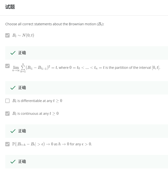
Week 4.6: Two definitions of a Brownian motion

Brownian Motion 又稱 Wiener process
[Brownian Motion Def1]:
We say that $B_t$ is Brownian motion if and only if
$B_t$ is a Gaussin process with $m(t)=0$ and $K(t,s)=\min(t,s)$

[Brownian Motion Def2]:
We say that $B_t$ is Brownian motion if and only if
$(0)$ $B_0=0$ almost surely (a.s.)
$(1)$ $B_t$ is independent increaments, i.e.
$\forall t_0<t_1<...<t_n$, we have $B_{t_1}-B_{t_0}, ..., B_{t_n}-B_{t_{n-1}}$ are independent
$(2)$ $B_t-B_s\sim\mathcal{N}(0,t-s)$, $\forall t>s\geq0$

[證明 Def1 $\Rightarrow$ Def2]:
先證明 $(0)$, 我們知道 $\mathbb{E}B_0 = m(0)=0$, $Var(B_0)=K(B_0, B_0)=0$
所以 $B_0=0$ a.s.
再來證明 $(1)$: $B_b-B_a \perp B_d-B_c, \forall 0\leq a\leq b\leq c\leq d$
我們先證明它們是 uncorrelated
$$Cov(B_b-B_a, B_d-B_c) \\ =Cov(B_b,B_d) - Cov(Ba,B_d) - Cov(B_b,B_c) + Cov(B_a,B_c) \\ = b-a-b+a = 0$$
所以 $B_b-B_a$ uncorrelated with $B_d-B_c$
之前我們學過, 如果 $(B_b-B_a, B_d-B_c)$ 是 Gaussian vector 的話
uncorrelated 等同於 independent
所以我們用 Gaussian vector 的定義來證明:
$$\lambda_1(B_b-B_a)+\lambda_2(B_d-B_c) \\ = \lambda_1B_b-\lambda_1B_a+\lambda_2B_d-\lambda_2B_c \\ \text{by Def1 }\sim \mathcal{N}$$
證得 $(B_b-B_a, B_d-B_c)$ 是 Gaussian vector 且已證過 uncorrelated, 所以 independent
最後證明 $(2)$:
首先 $B_t-B_s\sim\mathcal{N}$, 因為 by Def1 $B_t$ is Gaussian process, 所以線性組合也是 Gaussian
$\mathbb{E}[B_t-B_s]=\mathbb{E}[B_t]-\mathbb{E}[B_s]=m(t)-m(s)=0$
$$Var[B_t-B_s]=Cov(B_t-B_s,B_t-B_s) \\ = Cov(B_t,B_t)-2Cov(B_t,B_s)+Cov(B_s,B_s) \\ = t-s$$
Q.E.D.

[證明 Def2 $\Rightarrow$ Def1]:
我們先證明是 Gaussian process, $\forall t_1<t_2<...<t_n$ 考慮
$$\sum_{k=1}^n \lambda_k B_{t_k} = \lambda_n(B_{t_n}-B_{t_{n-1}}) + (\lambda_n+\lambda_{n-1})B_{t_{n-1}} + \sum_{k=1}^{n-2} \lambda_k B_{t_k} \\ = \sum_{k=1}^n d_k(B_{t_n}-B_{t_{n-1}}) \\ \text{by sum of independent Guassian is also Gaussian} \sim \mathcal{N}$$
所以 $(B_{t_1},...,B_{t_n})$ 是 Gaussian vector implies that $B_t$ 是 Gaussian process
是 Gaussian process 後, 我們找一下 $m(t),K(t,s)$
首先注意到我們有 $B_t=B_t-B_0\sim\mathcal{N}(0,t)$
所以 $m(t)=\mathbb{E}B_t=0$
接著計算 $K(t,s)$, for $t>s$
$$K(t,s)=Cov(B_t,B_s) \\ = Cov(B_t-B_s+B_s,B_s) \\ = Cov(B_t-B_s, B_s) + Cov(B_s,B_s) \\ = Cov(B_t-B_s, B_s-B_0) + s \\ \text{by indep. increment }= 0 + s = s$$
如果 $t<s$ 則 $K(t,s)=t$, 因此
$K(t,s)=\min(t,s)$
Q.E.D.

由 Brownian motion 的 Def2 我們可以推出一些東西:
For $t>s\geq0$, $B_t\sim\mathcal{N}(0,t)$, $B_s\sim\mathcal{N}(0,s)$, $B_{t-s}\sim\mathcal{N}(0,t-s)$
由 independent increament 知道 $B_{t-s}\perp B_s$, 又因為獨立 normal r.v.s 相加也仍是 normal, 且其 mean and variance 為直接相加
所以
$(B_{t-s}+B_s)\sim\mathcal{N}(0,t-s+s)=\mathcal{N}(0,t)=^d B_t \\$
$B_t(x)=B_{t-s}(x)+B_s(x)$

Week 4.7: Modification of a process. Kolmogorov continuity theorem

[Stochastically Equivalent Def]:
$X_t,Y_t$ are called stochastically equivalent if
$\mathcal{P}\{X_t=Y_t\}=1,\forall t\geq0$

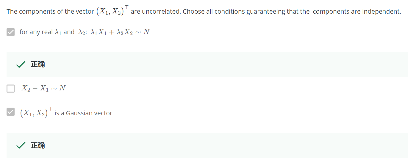
[Example]: stochastically equivalent 但行為卻不一樣的 r.v.s
$X_t=0,\forall t\in[0,1]$. And $Y_t=\mathbf{1}\{\tau=t\},\tau\sim Unif(0,1)$
在看 $Y_t$ 這個 random variable 的時候, $t$ 是給定的 (fixed), 而它的值只有可能是 $0$ or $1$
則很顯然 $X_t$ 和 $Y_t$ 是 stochastically equivalent:
$\mathcal{P}\{X_t=Y_t\}=\mathcal{P}\{Y_t=0\}=\mathcal{P}\{t\neq\tau\}=1$
我們劃出 $X_t$ 和 $Y_t$ 的 trajectory (參考 Week1 Introduction & Renewal process):
Stochastic process $X_t:\Omega\times\mathbb{R}_+\rightarrow\mathbb{R}$
Trajectory of an given outcome $\omega$, $X_t(\omega):\mathbb{R}_+\rightarrow\mathbb{R}$

圖中的 $x$-axis 為時間 $t$, $y$-axis 為 outcome 值經過 measurable function $X_t$ or $Y_t$ mapping 到的 real number (注意到 random variable 其實是個 measurable function)
上圖顯示了給定某一個 $t$, $X_t$ 和 $Y_t$ 的一條 trajectory

所以 trajectory 就是對某一個 outcome $\omega$ 經過 random variable $X_t$ mapping 後的那個數值隨著時間的變化.

對於所有的 $t$, $X_t(\omega)$ 都長一個樣, 而 $Y_t(\omega)$ 都長不一樣, 且都不連續

所以 $X_t$ 和 $Y_t$ 是 stochastically equivalent 但是 $X_t$ trajectory 是 continuous 而 $Y_t$ 不是
有沒有可能把一個 trajectory 不連續的 stochastic process 找道其對應 stochastically equivalent 的 process 呢 ?

[Kolmogorov continuity Theorem]:
Let $X_t$ be a stochastic process, if $\exists C,\alpha,\beta>0$ such that
$\mathbb{E}\left[ |X_t-X_s|^\alpha \right] \leq C\cdot |t-s|^{1+\beta},\forall t,s\in[a,b]$
then $\exists Y_t$ is stochastically equivalent to $X_t$ and $Y_t$ has continuous trajectories
We can say that the process $X_t$ has a continuous modification.

感覺有點像在說 trajectory 這個 function (x-axis 為時間, y-axis 為固定某個 outcome $\omega$ 經過 random variable mapping 的值, e.g. $X_t(\omega)$) 是 $C$-Lipschitz continuity

[Brownian motion has continuous modification]:
Let $B_t$ be a Brownian motion
We know that $B_t-B_s\sim\mathcal{N}(0,t-s)$, which also means
$B_t-B_s=^d\sqrt{t-s}\cdot\xi,\xi\sim\mathcal{N}(0,1)$
Then (using the 4-th moment of normal distribution)
$\mathbb{E}\left[ |B_t-B_s|^4 \right] = (t-s)^2\mathbb{E}\xi^4= (t-s)^2\cdot3$
We can see that it fullfilled Kolmogorov continuity Theorem
Conclude that Brownian motion has continuous modification.

一般我們稱 Brownian motion 都預設稱這個 continuous modification

Week 4.8: Main properties of Brownian motion

[Quadratic Variation Def]: wiki
$X_{t}$ is a stochastic process. It’s quadratic variation is the process, written as $[X_t]$, defined as
$[X_t]=\lim_{|\Delta|\rightarrow0}\sum_{k=1}^n (X_{t_k}-X_{t_{k-1}})^2$
where $\Delta:0=t_0<t_1<...<t_n=t$, is a partition, and $|\Delta|=\max_{i=1,...,n}\{t_i-t_{i-1}\}$
This limit, if it exists, is defined using convergence in probability (See Week 6 的開頭).

課程沒提供證明, 說在很多 stochastic 的書都有提供了

[Quadratic Variation of Brownian Motion]:
給一個 Brownian motion $B_t$, 考慮一個 partition $\bigtriangleup:0=t_0<t_1<...<t_n=t$
我們稱該 partition 的 quadratic variation 為以下 limit:
$\lim_{|\bigtriangleup|\rightarrow0} \sum_{k=1}^n\left( B_{t_k}-B_{t_{k-1}} \right)^2 = t$
$|\bigtriangleup|\rightarrow0$ 表示:$\max_{k=0,...,n}\{|t_k-t_{k-1}|\}\rightarrow0, \text{ for }n\rightarrow0$
從上面可以看出 Brownian motion 的 quadratic variation 極限值存在且等於 $t$
[Proof]:
使用 convergence in mean square sense 證明.
因為我們知道 m.sq. sense 成立則 converges in probability
(quadratic variation 的 limit 定義) 也成立. 更多參考 Week 6 開頭.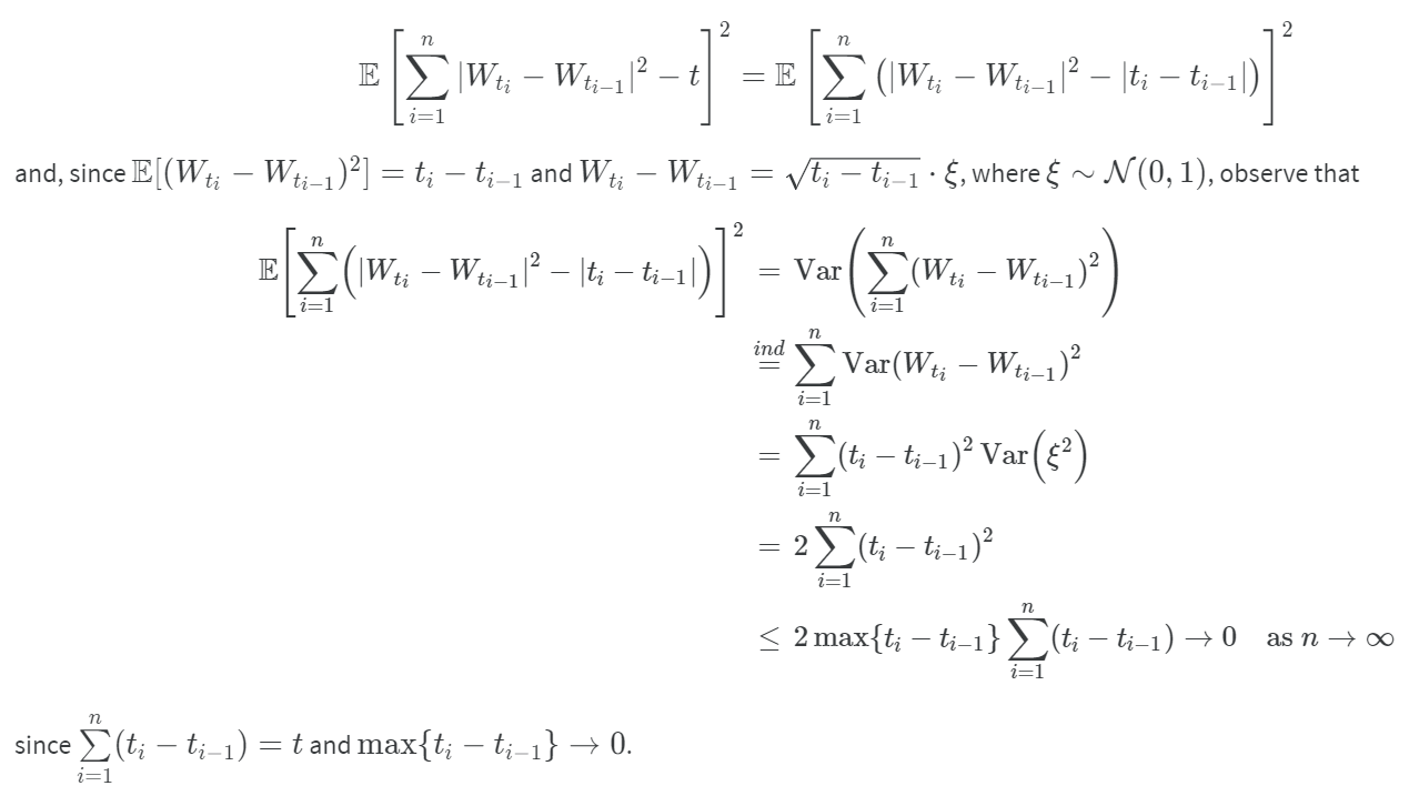

如果我們令:
$S_n=\sum_{k=1}^n\left( B_{t_k}-B_{t_{k-1}} \right)^2$
則 quadratic variation 告訴我們
$\mathbb{E}(S_n-t)^2\rightarrow0, \text{ for }n\rightarrow\infty$

[Variation of Brownian Motion]:
給一個 Brownian motion $B_t$, 考慮一個 partition $\bigtriangleup:0=t_0<t_1<...<t_n=t$
我們稱該 partition 的 variation 為以下 limit:
$\lim_{|\bigtriangleup|\rightarrow0} \sum_{k=1}^n | B_{t_k}-B_{t_{k-1}} | = \infty$
從上面可以看出 Brownian motion 的 variation 極限值不存在

課程說 variation 不存在的證明會用到 quadratic variation 存在的定理, 但沒給證明

總結來說, Brownian motion 是 quadratic variation, 但不是 bounded variation

[Brownian Motion Continuity and Differentiability]:
Brownian motion is everywhere continuous but nonwhere differentiable.
我們說 stochastic process 是 continuous at time $t$ 意思為:
$$B_{t+h}\xrightarrow[h\rightarrow0]{p}B_t \\ \Longleftrightarrow\mathcal{P}\{|B_{t+h}-B_t|>\varepsilon\}=0, \text{ for }h\rightarrow0, \forall\varepsilon>0$$
而 differentiable 會在 week6 提到.

接下來的定理可以用來了解 Brownian motion $B_t$ 跑向 $\infty$ 的速度有多快.
$$\begin{align} \begin{array}{rl} \lim_{t\rightarrow\infty}\frac{B_t}{t}=0, &a.s. \\ \lim\sup_{t\rightarrow\infty}\frac{B_t}{\sqrt{t}}=\infty, &a.s. \end{array} \end{align}$$

課程說很容易證明… 但對我來說不是 (Law of the iterated logarithm)

直觀理解為: Brownian motion 跑得比 $t$ 還慢, 但是比 $\sqrt{t}$ 還快
但準確來說 Brownian motion 的速度應該是什麼? Law of the Iterated Logarithm 告訴了我們答案

[Law of the Iterated Logarithm]:
Brownian motion $B_t$, we have
$\lim\sup_{t\rightarrow\infty} \frac{B_t}{\sqrt{2t\log(\log t)}}=1$

無法太深入理解這些定理的用處和意義, 同意課程要給更多範例說明

最後一個問題可以由 $\lim_{h\rightarrow0} B_{t+h}-B_t \sim \lim_{h\rightarrow0}\mathcal{N}(0,h)$ 看出, 為 constant $0$ a.s.

END OF CLASS