Stochastic Processes Week 6 Ergodicity, differentiability, continuity

---

Coursera Stochastic Processes 課程筆記, 共十篇:

• Week 0: 一些預備知識
• Week 1: Introduction & Renewal processes
• Week 2: Poisson Processes
• Week3: Markov Chains
• Week 4: Gaussian Processes
• Week 5: Stationarity and Linear filters
• Week 6: Ergodicity, differentiability, continuity (本文)
• Week 7: Stochastic integration & Itô formula
• Week 8: Lévy processes
• 整理隨機過程的連續性、微分、積分和Brownian Motion

---

Self Study: Convergence of random variables

主要參考 wikipedia 的資料筆記 Convergence of random variables
[Converge in distribution Def]: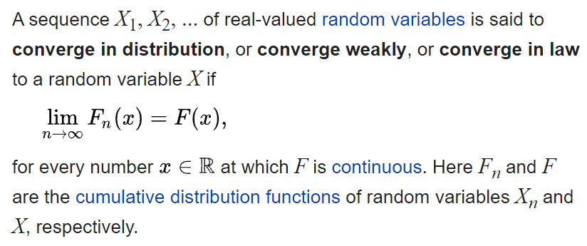

 記做 $X_n \xrightarrow[]{d}X$

Converge in distribution 是最 weak 的, 也就是滿足 converge in distribution 不一定會滿足 converge in probability 或滿足 almost surely 或滿足 converge in mean
[機率論] 兩隨機變數相等表示兩者有相同分布但反之不然, 這篇文章最後給了一個例子:
考慮均勻分布 $X$ 為隨機變數服從均勻分布 $\mathcal{U}[-1,1]$ 現在取另一隨機變數 $Y:=-X$ 則 $Y$ 亦為在 $[-1,1]$ 上均勻分布，亦即 $X$ 與 $Y$ 具有同分布。然而
$\mathcal{P}(X=Y)=0$

Converge in distribution 的其他等價定義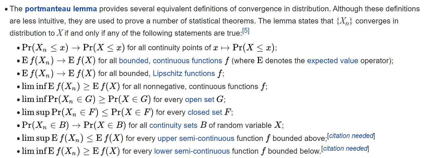

[Converge in probability Def]: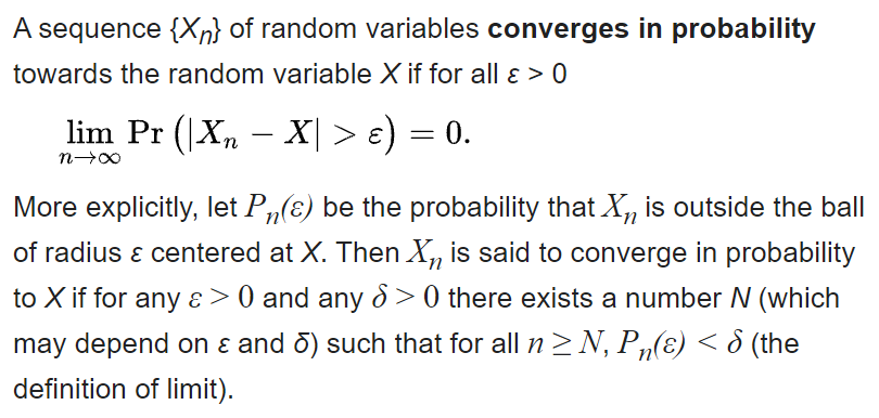

 記做 $X_n \xrightarrow[]{p}X$

[Properties]: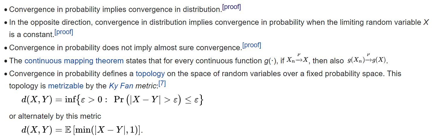

自己的想法: $X_n$ 與 $X$ 的 sample spaces 可以不同, 只要 mapping 到 $\mathbb{R}$ 之後相減就好, 所以考量的是 joint distribution
For a random process $X_t$ converges to a constant in probability sense
$X_t\xrightarrow[t\rightarrow\infty]{p} c \text{ (is const.)}$
則表示一定會 (必要條件)

$$\mathbb{E}X_t\xrightarrow[t\rightarrow\infty]{}c \\ Var(X_t)\xrightarrow[t\rightarrow\infty]{}0$$

[Almost sure convergence Def]: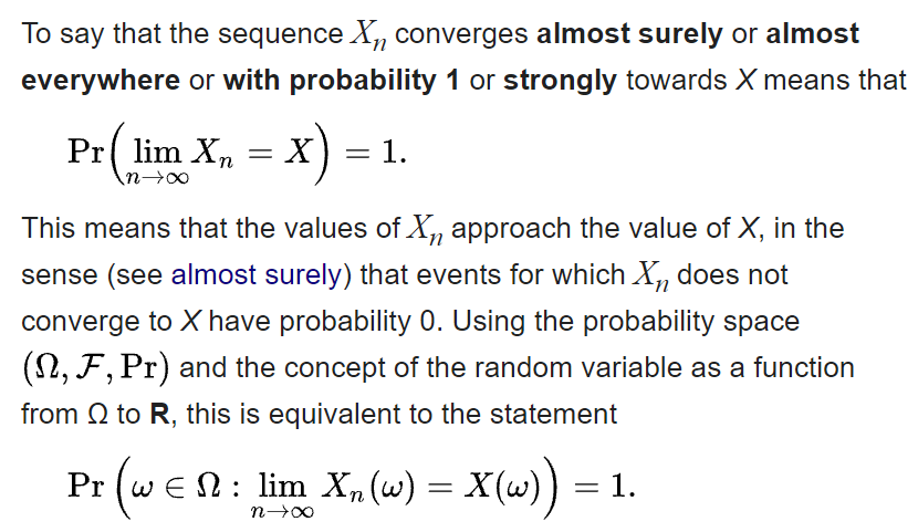

 記做 $X_n \xrightarrow[]{a.s.} X$

可參考: 謝宗翰的隨筆 [機率論] Almost Sure Convergence

自己的想法: 需要 sample space 一樣, 且都是對個別 outcome 去比較的. 把所有這些符合的 outcomes 蒐集起來的集合, 其 probability measure 為 $1$.
這是一個很強的條件, 幾乎針對每一個 outcome 都要符合.

[Convergence in mean Def]: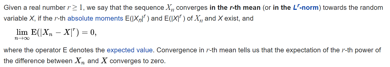


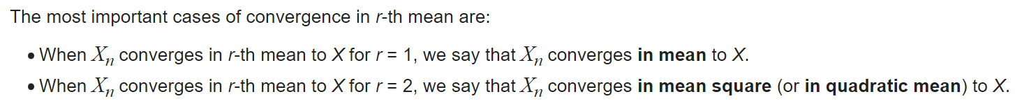
 記做 $X_n \xrightarrow[]{L^r} X$.

Convergence in the $r$-th mean, for $r\geq1$, implies convergence in probability (by Markov’s inequality). Furthermore, if $r>s\geq1$, convergence in $r$-th mean implies convergence in $s$-th mean. Hence, convergence in mean square implies convergence in mean.
It is also worth noticing that if

$$X_n\xrightarrow[]{L^r}X$$

then

$$\lim_{n\rightarrow\infty}\mathbb{E}[|X_n|^r]=\mathbb{E}[|X|^r]$$

[Relation btw Stochastic Convergences]: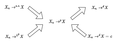

• 各種 convergence 的 proofs:
  https://en.wikipedia.org/wiki/Proofs_of_convergence_of_random_variables#propA2

補上課程針對以上四個 convergences 的定義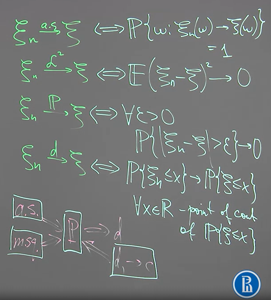

---

Week 6.1: Notion of ergodicity. Examples

Motivated by LLN (Law of Large Number)
[LLN Thm]:
 $\xi_1,\xi_2,…$ - i.i.d. and $\mathbb{E}\xi_1<\infty$, then
 $\frac{1}{N}\sum_{n=1}^N \xi_n \xrightarrow[N\rightarrow\infty]{p} \mathbb{E}\xi_1$
 上式 $\xrightarrow[]{p}$ 表示 convergence in probability
 但也滿足 $\xrightarrow[]{a.s.}$ almost sure convergence (Strong LLN)

Ergodicity 嘗試將 LLN 概念延伸到 stochastic process

[Ergodicity Def]:
 $X_t$ is a stochastic process, where $t=1,2,3,…$
 $X_t$ is said ergodic if $\exists c$ constant such that
 

$$M_T:=\frac{1}{T}\sum_{t=1}^T X_t \xrightarrow[T\rightarrow\infty]{p} c$$
 where $c$ is some constant. $T$ is called horizon.
 And we consider convergence in probability sense.

所以要證明 ergodic 可以 $\xrightarrow[]{p}$, or $\xrightarrow[]{a.s.}$, or $\xrightarrow[]{m.sq.}$, or $\xrightarrow[]{d}c$

[Example 1]:
 $X_t=\xi\sim\mathcal{N}(0,1)$, trajectory 為 constant for all $t$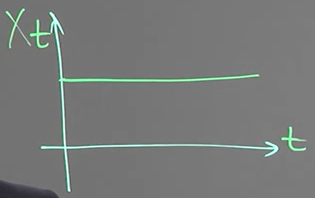

 $m(t)=0,K(t,s)=Var\xi=1$
 所以是 weak stationary, 我們考慮 ergodicity
 $\frac{1}{T}\sum_{t=1}^T X_t=\xi\neq c$
 不存在一個 constant for $T\rightarrow \infty$, 所以 non-ergodic

[Example 2]:
 $X_t$ stochastic process defined as:
 $X_t=\varepsilon_t+a\cos\frac{\pi t}{6}$
 where $a\neq0$ and $\varepsilon_1, \varepsilon_2, …$ i.i.d. $\mathcal{N}(0,1)$

其 trajectory 為下圖曲線, 並對該曲線每個位置都有 std normal noise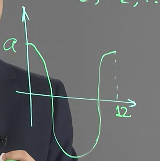


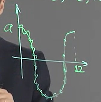
$m(t)=a\cos\frac{\pi t}{6}\neq const$, 所以不是 stationary. 考慮 ergodicity:
$\frac{1}{T}\sum_{t=1}^T X_t\sim\mathcal{N}\left(\frac{a}{T}\sum_{t=1}^T \cos\frac{\pi t}{6},\frac{1}{T}\right)$
互相獨立之 normal distributions 相加仍為 normal, mean and variance 都為相加
variance 收斂到 $0$, 觀察 mean:
由於 trajectory 是以 12 為一個週期, 所以最多只會有 12 個非 0 的值, 而每一個都小於等於 1
結論是 mean 也收斂到 $0$ (因為不管哪一個 outcome, 其 trajectory 最後都到 $0$, 所以收斂的 random variable 為 contant $0$)
所以
$\frac{1}{T}\sum_{t=1}^T X_t\sim\mathcal{N}\left(0,0\right) \text{ for }T\rightarrow\infty$
所以 $=0$ a.s. 因此是 ergodic
Example 1 是 (weak) stationary but non-ergodic
Example 2 是 non-stationary but erogodic
因此 stationary 跟 ergodic 是不同概念

---

Week 6.2: Ergodicity of wide-sense stationary processes

[Proposition]:
For $X_t$ is a discrete time stochastic process. Define
 

$$M_T=\frac{1}{T}\sum_{t=1}^TX_t\\ C(T)=Cov(X_T,M_T)$$
 If $\exists\alpha$ such that the covariance function is bounded by $\alpha$, i.e.
 $|K(s,t)|\leq\alpha;\forall s,t$
 Then
  $$Var(M_T)\xrightarrow[T\rightarrow\infty]{}0 \Longleftrightarrow C(T)\xrightarrow[T\rightarrow\infty]{}0$$

[Stolz-Cesaro Thm]:
  For $a_n,b_n\in\mathbb{R}$, $b_n$ is strictly increasing and unbounded, we have:
 $\lim_{n\rightarrow\infty}\frac{a_n-a_{n-1}}{b_n-b_{n-1}}=q\Longrightarrow \frac{a_n}{b_n}\xrightarrow[n\rightarrow\infty]{}q$

See wiki for more detials and proof

當 stationary 時, 有兩個 sufficient conditions 滿足則保證 ergodic
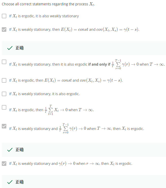
[Sufficient Conditions of Ergodicity when WSS]:
 $X_t$ is weakly stationary and $\gamma(\cdot)$ is its auto-covariance function with $|\gamma(\cdot)|<\infty$.
 1. Sufficient condition: If
  $\frac{1}{T}\sum_{r=0}^{T-1}\gamma(r) \xrightarrow[T\rightarrow\infty]{}0$
  Then $X_t$ is ergodic
 2. Sufficient condition: If
  $\gamma(r) \xrightarrow[r\rightarrow\infty]{}0$
  Then $X_t$ is ergodic
[Proof 1]:
 考慮 $C(T)$
 

$$C(T)=Cov\left(X_T,\frac{1}{T}\sum_{t=1}^TX_t\right) =\frac{1}{T}\sum_{t=1}^T Cov(X_T,X_t) \\ =\frac{1}{T}\sum_{t=1}^T \gamma(T-t) =\frac{1}{T}\sum_{r=0}^{T-1}\gamma(r) \longrightarrow0\text{ (by assumption)}$$
 由 proposition 知道 $Var(M_T)\rightarrow0$, as $T\rightarrow\infty$
 又因為已知 $X_t$ is weakly stationary, 所以 $\exists c$ constant, s.t.
 $\mathbb{E}X_t=c\Rightarrow\mathbb{E}M_t=c$
 則 variance converge to $0$ as $T\rightarrow\infty$ 表示
 $VarM_T=\mathbb{E}\left[(M_T-c)^2\right]\xrightarrow[T\rightarrow\infty]{}0$
 則
 $M_T \xrightarrow[]{L^2} c \Longrightarrow M_T \xrightarrow[]{p} c$
 根據定義 $X_t$ is ergodic. Q.E.D.

[Proof 2]:
 我們利用 proof 1 的結果和 Stolz-Cesaro thm, 定義
 

$$a_n:=\sum_{r=0}^{n-1}\gamma(r)\\ b_n:=n$$
 則
  $$\frac{a_n-a_{n-1}}{b_n-b_{n-1}}=\frac{\gamma(n-1)}{1}\xrightarrow[n\rightarrow\infty]{}0=q \\ \Longrightarrow \frac{a_n}{b_n} = \frac{1}{n}\sum_{r=0}^{n-1}\gamma(r)\xrightarrow[n\rightarrow\infty]{}0=q \\ \Longrightarrow X_t \text{ ergodic}$$

[Example 1]:
 $N_t$ is Poisson process with $\lambda$. 給定 $p>0$, 並定義
 $X_t:=N_{t+p}-N_t$
 則我們可得知 $X_t$ is ergodic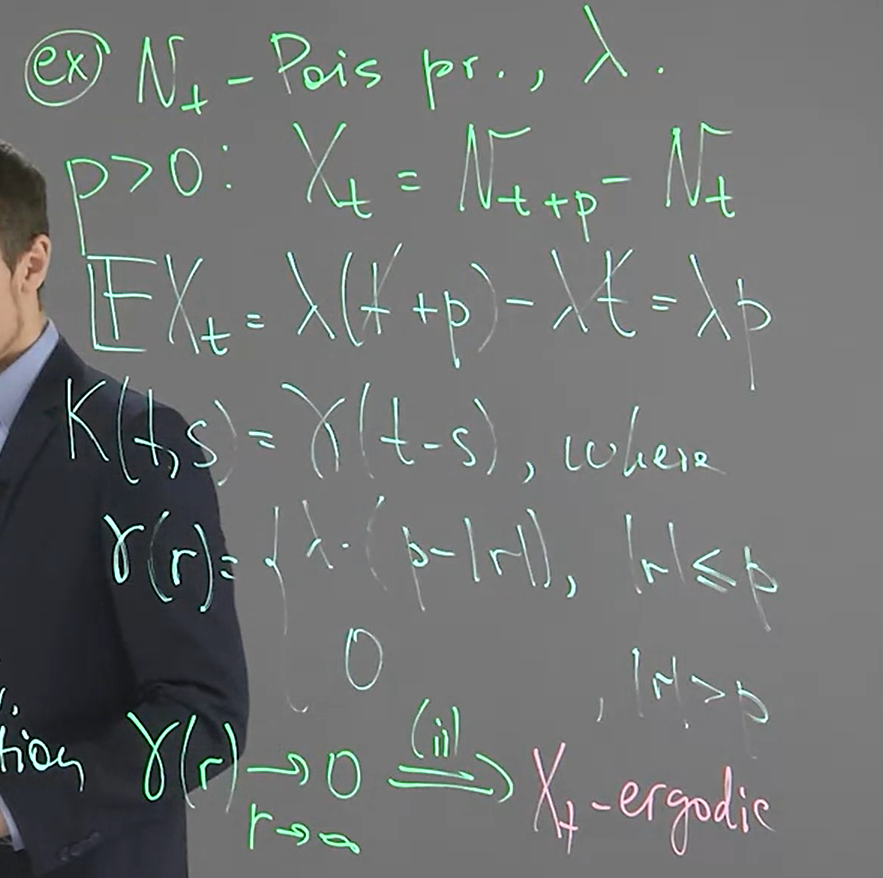

You can use the independent increment property of Poisson Process to get this formula.
$\gamma(t-s) = Cov(N_{t+p}-N_t,N_{s+p}-N_s)$
If $|s-t|>p$, then $N_{t+p}-N_t$ is independent of $N_{s+p}-N_s$, so $\gamma(t-s)=0$
If $t<s<t+p$, then $N_t$ is independent of $N_{s+p}-N_s$, so

$$Cov(N_{t+p}-N_t,N_{s+p}-N_s) = Cov(N_{t+p},N_{s+p}-N_s) \\ = Cov(N_{t+p},N_{s+p}) - Cov(N_{t+p},N_s) \\ = Cov(N_{t+p},N_{s+p} - N_{t+p} + N_{t+p}) - Cov(N_{t+p} - N_s + N_s,N_s) \\ = Var(N_{t+p}) - Var(N_s) = \lambda(t+p-s)$$
For $s<t<s+p$. you can deal with it similarly.

[Example 2]:
 $A,B$ 都是 r.v.s 有如下圖的 expectation and uncorrelated relation
 $\omega$ 是任意給定的 fixed value
 則我們發現 $X_t$ is weakly stationary and ergodic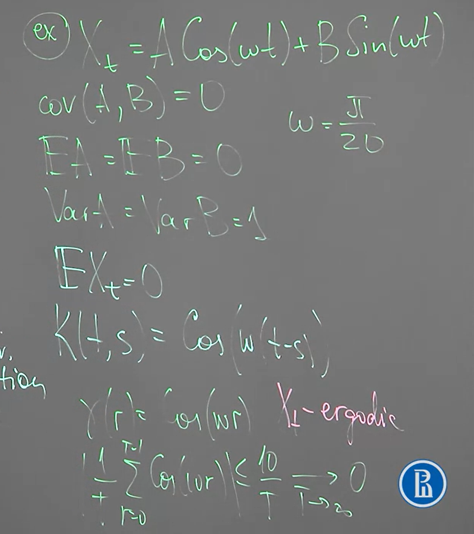

---

Week 6.3: Definition of a stochastic derivative

[Stochastic Derivative Def]:
 We say that a random process $X_t$ is differentiable at $t=t_0$
 if the following limit converges in m.sq. sense to some random variable $\eta$
 $\frac{X_{t+h}-X_t}{h} \xrightarrow[h\rightarrow0]{L^2}\eta:=X_{t_0}'$
 equivalently we can write as follows
 $\mathbb{E}\left[\left(\frac{X_{t+h}-X_t}{h}-\eta\right)^2\right] \xrightarrow[h\rightarrow0]{}0$

[Proposition, Differentiability of Stochastic Process]:
 Let $X_t$ is a stochastic process and $\mathbb{E}X_t^2<\infty$.
 Then $X_t$ is differentiable at $t=t_0$ if and only if
 

$$\exists\frac{dm(t)}{dt}\text{, at }t=t_0 \\ \exists\frac{\partial}{\partial t\partial s}K(t,s)\text{, at }(t_0,t_0)$$

[Brownian Motion is NOT differentiable at any time $t$]: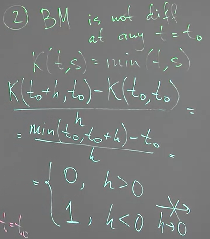

[Differentiability of Independent Increments]:
 $X_t$ is independent increments and $X_0=0$ a.s. 則我們知道
 $K(t,s)=Var(X_{\min(t,s)})$
 因此大部分的 stochastic process with independent increments 都不是可微的.
 我們寫一下 covariance function 的推導:
 

$$K(t,s)=Cov(X_t,X_s) \\ \text{(for t>s) }=Cov(X_t-X_s,X_s-X_0)+Cov(X_s,X_s) \\ = 0+Var(X_s)\\ \text{(consider t>s and t<s) }= Var(X_{\min(t,s)})$$

[Differentiability of Weakly Stationary]:
 $X_t$ is weakly stationary. 所以 $m(t)$ is constant $\Rightarrow$ differentiable at all $t$.
 我們知道 $K(t,s)=\gamma(t-s)$, 計算 partial derivatives:
 

$$\left.\frac{\partial^2K(t,s)}{\partial t\partial s} \right\vert_{(t_0,t_0)} = \frac{\partial^2 \gamma(t-s) }{\partial t\partial s} \\ = \left.\frac{\partial}{\partial t} \left(-\gamma'(t-s)\right)\right|_{(t_0,t_0)} = \left.-\gamma''(t-s)\right|_{(t_0,t_0)} \\ = -\gamma''(0)$$
 所以 $X_t$ is differentiable (at any time $t$) if and only if $-\gamma’’(0)$ 存在

[Example 1]:
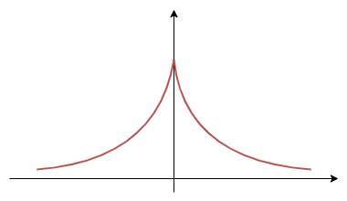
 承上 weakly stationary differentiable. 如果 $\gamma(r)=e^{-\alpha|r|}$
 則 $X_t$ is not differentiable, 因為 $-\gamma’’(0)$ 不存在 ($\gamma’(0)$ 就不存在了). $\gamma(t)$ 如下:

[Example 2]:
 承上 weakly stationary differentiable. 如果 $\gamma(r)=\cos(\alpha r)$
 則 $X_t$ is differentiable

---

Week 6.4: Continuity in the mean-squared sense

[Continuity in the probability sense Def]:
 $X_t\xrightarrow[t\rightarrow t_0]{p}X_{t_0} \Longleftrightarrow \mathcal{P}(|X_t-X_{t_0}|>\varepsilon)\xrightarrow[t\rightarrow t_0]{}0, \qquad \forall\varepsilon>0$

Converges in mean-squared sense 確保了 converges in probability, 且 in m.sq. sense 比較容易確認, 因此以下著重在 in m.sq. sense

[Continuity in the mean-squared sense Def]:
 $X_t\xrightarrow[t\rightarrow t_0]{L^2}X_{t_0} \Longleftrightarrow \mathbb{E}(X_t-X_{t_0})^2\xrightarrow[t\rightarrow t_0]{}0$

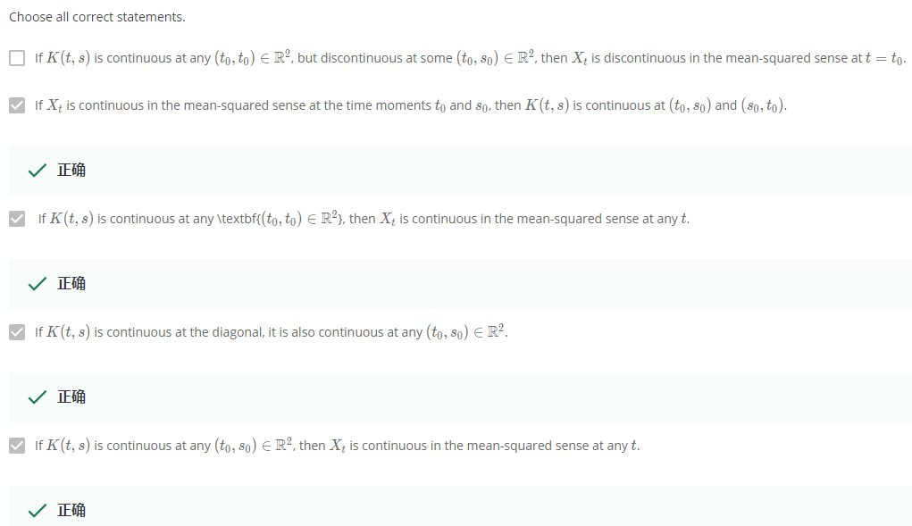
[Proposition, Continuity of Stochastic Process]:
 $X_t$ stochastic process and $\mathbb{E}X_t=0$
 1. If $K(t,s)$ is continuous at $(t_0, t_0)$, then $X_t$ is continuous in the m.sq. sense at $t=t_0$
 2. If $X_t$ is continuous in the m.sq. sense at $t=t_0,s_0$, then $K(t,s)$ is continuous at $(t_0,s_0)$

[Proof 1]:
 proved by definition of m.sq. sense
 

$$\mathbb{E}(X_t-X_{t_0})^2 = \mathbb{E}X_t^2-2\mathbb{E}X_tX_{t_0} + \mathbb{E}X_{t_0}^2 \\ =K(t,t)-2K(t,t_0)+K(t_0,t_0)\xrightarrow[t\rightarrow t_0]{}0$$
[Proof 2]:
  $$K(t,s)-K(t_0,s_0) \\ = (K(t,s)-K(t_0,s)) + (K(t_0,s) - K(t_0,s_0))$$
 使用 $\mathbb{E}X_t=0$ and 科西不等式, 考慮第一項 $K(t,s)-K(t_0,s)$
  $$|K(t,s)-K(t_0,s)|=|\mathbb{E}[(X_t-X_{t_0})X_s]| \\ \leq \sqrt{\mathbb{E}(X_t-X_{t_0})^2}\cdot\sqrt{\mathbb{E}X_s^2}\\ \text{by assumption }\xrightarrow[t\rightarrow t_0]{}0$$
 第二項 $K(t_0,s) - K(t_0,s_0)$ 也一樣. Q.E.D.

Differentiability 要關注 $m(t)$ and $K(t,s)$ 的微分性, 而 continuity 只關注 $K(t,s)$ 的連續性
另外對於 simplest type of stochastic integral $\int X_tdx$ 來說, 關注的是 $m(t)$ and $K(t,s)$ 的連續性

[Corollary]:
 Covariance function $K(t,s)$ is continuous at $(t_0,s_0),\forall t_0,s_0$ if and only if
 $K(t,s)$ is continuous at diagonal, i.e. $(t_0,t_0),\forall t_0$

[Proof]:
 只需證明 $\Longleftarrow$
 $K(t,s)$ is continuous at $(t_0,t_0)$, $\forall t_0$. 由 proposition 1 知道 $X_t$ is continuous in m.sq. sense $\forall t$
 因此 $X_t$ is continuous in the m.sq. sense at $t=t_0,s_0$ for all points
 由 proposition 2 知道 $K(t,s)$ is continuous at $(t_0,s_0),\forall t_0,s_0$
 Q.E.D.