Coursera Stochastic Processes 課程筆記, 共十篇:
- Week 0: 一些預備知識
- Week 1: Introduction & Renewal processes
- Week 2: Poisson Processes
- Week3: Markov Chains
- Week 4: Gaussian Processes
- Week 5: Stationarity and Linear filters
- Week 6: Ergodicity, differentiability, continuity
- Week 7: Stochastic integration & Itô formula (本文)
- Week 8: Lévy processes
- 整理隨機過程的連續性、微分、積分和Brownian Motion
四種 types 的 stochastic integration, where $X_t,H_t$ are stochastic processes, $f(t)\in L^2([a,b])$ is a deterministic function, $W_t$ is a Brownian motion, and $a,b\in\mathbb{R}$
$$\begin{align}
\int_a^b X_t dt \\
\int_a^b f(t)dW_t \\
\int_a^b X_t dW_t \\
\int_a^b X_t dH_t
\end{align}$$
在 stochastic integral 跟以往的 integral 很不一樣的一點是, 我們發現 integral 的結果仍然是一個 random variable
閱讀以下內容時可以看出這一點
Week 7.1: Different types of stochastic integrals. Integrals of the type $∫ X_t dt$
Given a Stochastic process $X_t:\Omega\times\mathbb{R}_+\rightarrow\mathbb{R}$
如果我們固定一個 outcome $\omega$, 則 $X_t(\omega):\mathbb{R}_+\rightarrow\mathbb{R}$, 因此我們就可以考慮 Riemann integral:
$\int_a^b X_t(\omega)dt=\color{orange}{\lim_{|\Delta|\rightarrow0}}\sum_{k=1}^n X_{t_{k-1}}(\omega)\cdot(t_k-t_{k-1})$
For partition $\Delta:a=t_0\leq t_1\leq …\leq t_n=b$, $|\Delta|=\max\{t_k-t_{k-1}\},k=1,...,n$
若考慮 stochastic process, 上述的 limit 必須以 mean square sense 來考慮, 因此正式定義如下:
[Stochastic Integrals of Simplest Type $∫ X_t dt$]:
Given a Stochastic process $X_t:\Omega\times\mathbb{R}_+\rightarrow\mathbb{R}$
Given partition $\Delta:a=t_0\leq t_1\leq ...\leq t_n=b$, $|\Delta|=\max\{t_k-t_{k-1}\},k=1,...,n$
If the following expectation converges to some value $A$ in mean square sense:
$$\mathbb{E}\left[
\left(
A - \sum_{k=1}^n X_{t_{k-1}}(t_k-t_{k-1})
\right)^2
\right]
\xrightarrow[|\Delta|\longrightarrow0]{} 0$$
Then we denote(define) the converged value $A$ as: $\int_a^b X_t dt$
[Existence of the Simplest Type of Stochastic Integral]:
$X_t:\mathbb{E}[X_t^2]<\infty$, if
1. $m(t)$ continuous
2. $K(t,s)$ continuous
Then the stochastic integral exists, i.e. $\int_a^b X_tdt<\infty$
有上述定理好處如下
We assume integral is taken in an bounded interval $[a,b]$
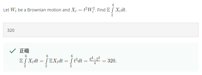
1. Expectation of stochastic integral:
$\mathbb{E}\left[ \int X_tdt \right] = \int \mathbb{E}[X_t]dt$
課程老師說 apply Frobenius theorem 可得此結果. 看不懂 Frobenius theorem
2. Expectation of squared stochastic integral:
$$\mathbb{E}\left[
\left(\int X_t dt\right)^2
\right] = \mathbb{E}\left[
\int\int X_t X_s dtds
\right] \\
= \int\int\mathbb{E}[X_tX_s]dtds$$
3. Variance of stochastic integral:
$$Var\left[
\int X_t dt
\right] = \mathbb{E}\left[
\left(\int X_t dt\right)^2
\right] - \left(\mathbb{E}\left[ \int X_tdt \right]\right)^2 \\
= \int\int \mathbb{E}[X_tX_s]dtds - \mathbb{E}\left[ \int X_tdt \right]\mathbb{E}\left[ \int X_sds \right]\\
= \int\int \mathbb{E}[X_tX_s]dtds - \int\mathbb{E}[X_t]dt\cdot\int\mathbb{E}[X_s]ds \\
= \int_a^b\int_a^b K(t,s) dtds \\
\because\text{symmetric}= 2\int_a^b \int_a^s K(t,s) dtds$$
注意到 $W_t\sim\mathcal{N}(0,t)$, 所以 $Var(W_t)=\mathbb{E}W_t^2=t$
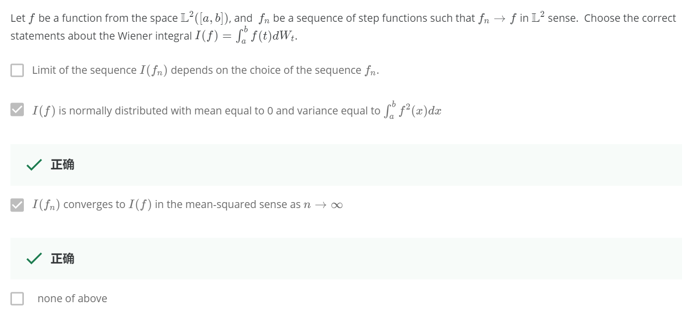
Week 7.2-3: Integrals of the type $∫ f(t) dW_t$
第二種 type 的 integral 我們稱為 Wiener integral
$\int_a^b f(t)dW_t$
where $f(t)\in L^2([a,b])$ is a deterministic function, $W_t$ is a Brownian motion, and $a,b\in\mathbb{R}$
[Inner Product in Function Space]:
Define inner product between real valued functions $f,g$ in $[a,b]$
$<f,g>=\int_a^b f(x)g(x)dx$
Having properties:
1. $<f,g>=<g,f>$
2. $<a_1f_1+a_2f_2,g>=a_1<f_1,g>+a_2<f_2,g>$
3. $<f,f>\geq0$, and $=0\Longleftrightarrow f=0$
[Informal Def of $L^2$ Space]:
定義 norm 為 $\|f\|_2 = \sqrt{<f,f>}$, 則所有 $\|f\|_2\leq\infty$ 所形成的空間
(搭配 $\|\cdot\|_2$ 則為 Banach space, 搭配 $<\cdot,\cdot>$ 則為 Helbert sapce) 我們稱為 $L^2$ space
比較嚴謹的定義參考數學課本
因此我們可以說在 $L^2$ space 上的收斂, 視為該 normed (Banach) space 上的收斂, i.e.
$$f_n\xrightarrow[]{L^2}f\Longleftrightarrow \|f_n-f\|_2\xrightarrow[n\rightarrow\infty]{}0 \\
\text{, or } \Longleftrightarrow \int_a^b \left( f_n(x)-f(x) \right)^2 dx
\xrightarrow[n\rightarrow\infty]{}0$$
我們先定義 Wiener integral of a step function
[Wiener Integral of a Step Function]:
Let $a=t_0\leq t_1\leq …\leq t_n=b$, $\alpha_i\in\mathbb{R}$, and step function $f(x)$ defined as:
$f(x)=\sum_{i=1}^n \alpha_i\cdot\mathbf{1}\{t_{i-1}\leq x<t_i\}$
Then Wiener integral of $f(x)$ is:
$\int_a^b f(x)dW_t = \sum_{i=1}^n \alpha_i\cdot(W_{t_i}-W_{t_{i-1}})$
[Example]: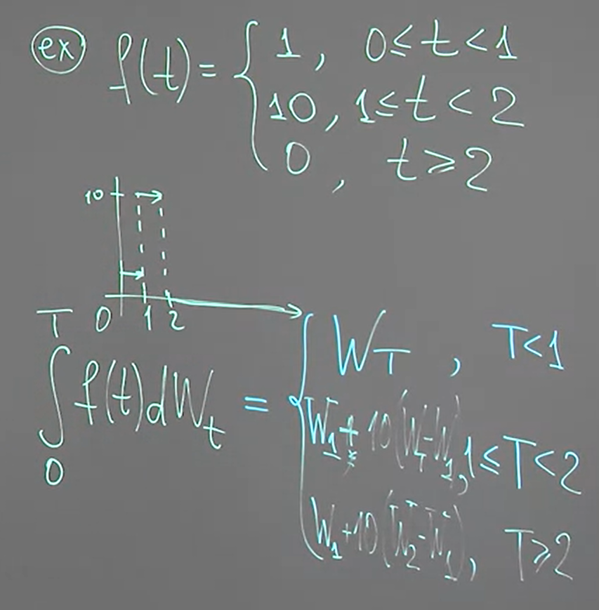
我們可以發現 integral 的結果都是 normal distribution
[Distribution of Wiener Integral of a Step Function]:
Let $f(x)$ is a step function, and Wiener integral as:
$I(f):=\int_a^b f(t)dW_t$
then
$I(f)\sim\mathcal{N}\left(0,\int_a^bf^2(x)dx\right)$
[Proof]:
根據 Wiener integral 的定義, 我們可以知道
$\int_a^b f(x)dW_t = \sum_{i=1}^n \alpha_i\cdot(W_{t_i}-W_{t_{i-1}})$
而因為 $W_t$ is Brownian motion, 具有 independent increment 性質
因此等於是互相獨立的 normal distribution 線性組合的結果, 所以也是 normal. 因此我們只需計算 mean and variance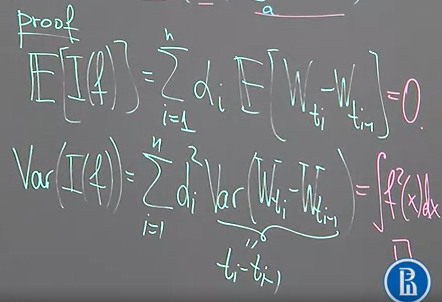
[Wiener Integral of a Deterministic $L^2$ Function]:
Let $f(x)\in L^2([a,b])$, and if we can find a sequence of step functions $(f_n)_n$
such that converges to $f$ in $L^2$ space, i.e.:
$f_n\xrightarrow[]{L^2}f\Longleftrightarrow \int_a^b\left( f_n(t)-f(t) \right)^2 dt \xrightarrow[n\rightarrow\infty]{}0$
then we define $I(f)$ as the limit of $I(f_n)$ as $n\rightarrow\infty$, i.e.:
$I(f):=\lim_{n\rightarrow\infty} I(f_n)$
Where the limit should be understood by mean square sense:
$$\mathbb{E}\left[
(I(f_n)-I(f))^2
\right] \xrightarrow[n\rightarrow\infty]{}0$$
觀察以上的定義, 有 3 個重要的問題需要回答:
- Why $I(f)$ doesn’t depend on $(f_n)_n$?
- Properties of $I(f)$?
- How to counstruct $(f_n)_n$? Will be answered in Week 7.4-5
[Theorem Explian Why $I(f)$ doesn’t depend on $(f_n)_n$]:
$(f_n)_n,(\tilde{f}_n)_n$ sequences of step functions in $L^2$ space and both converges to $f$, i.e.
$f_n\xrightarrow[]{L^2}f, \tilde{f}_n\xrightarrow[]{L^2}f$
Then
$\lim_{n\rightarrow\infty} I(f_n) = \lim_{n\rightarrow\infty} I(\tilde{f_n})$
The limit is understood as mean square sense, that is:
$$\mathbb{E}\left[
(I(f_n)-I(\tilde{f}_n))^2
\right] \xrightarrow[n\rightarrow\infty]{}0$$
Note that the Wiener integral of a step function $f$ is defined as:
$I(f):=\int_a^b f(t)dW_t$
and $W_t$ is Brownian motion
[Proof]:
$I(f_n)-I(\tilde{f}_n)=I(f_n-\tilde{f}_n)$ also is a step function
所以這個 step function 的 Wiener integral 會 follow normal distribution:
$I(f_n-\tilde{f}_n)\sim\mathcal{N}\left(0,\int_a^b (f_n(x)-\tilde{f}_n(x))^2 dx\right)$
所以 Variance:
$$Var(I(f_n-\tilde{f}_n)) = \mathbb{E}\left[
(I(f_n-\tilde{f}_n))^2
\right] \\
= \int_a^b (f_n(x)-\tilde{f}_n(x))^2 dx \xrightarrow[n\rightarrow\infty]{} 0$$
最後會 approach to $0$ 是因為 both converges to $f$.
所以馬上就發現 limit converges in mean square sense:
$$\because \mathbb{E}\left[
(I(f_n)-I(\tilde{f}_n))^2
\right] =
\mathbb{E}\left[
(I(f_n-\tilde{f}_n))^2
\right] \\
= Var(I(f_n-\tilde{f}_n)) \xrightarrow[n\rightarrow\infty]{}0
\\
\therefore\lim_{n\rightarrow\infty} I(f_n) = \lim_{n\rightarrow\infty} I(\tilde{f_n})$$
[The Wiener Integral of Function in $L^2$ Space]:
$\forall f\in L^2([a,b])$, The Wiener integral:
$I(f)\sim\mathcal{N}\left(0,\int_a^b f^2(x)dx\right)$
[Proof]:
For any $(f_n)_n$ converges to $f$ in $L^2$, we have
$$I(f)=\lim_{n\rightarrow\infty} I(f_n)\\
I(f_n)\sim\mathcal{N}\left(
0, \int_a^b f^2_n(x)dx
\right)$$
Normal distribution 的 limit 仍是 normal, 其結果為 mean and variance 的 limit, 所以
$$I(f)\sim\mathcal{N}\left(
0, \lim_{n\rightarrow\infty}\int_a^b f^2_n(x)dx
\right)
= \mathcal{N}\left(
0, \int_a^b f^2(x)dx \right)$$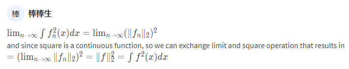
Q.E.D.
Week 7.4-5: Integrals of the type $∫ X_t dW_t$
要定義這樣的 integral, $X_t$ 必須定義在 filtered probability space 上.
[Filteration Def]: from Wiki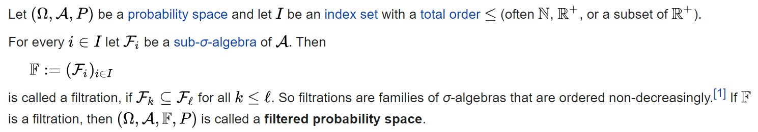
[Filteration Def]:
Filtration is a sequence of $\sigma$-algebras $\mathcal{F}_t$ defined on the same probability space $(\Omega,\mathcal{F},\mathcal{P})$
such that, $\mathcal{F}_t$ is a sub-$\sigma$-algebra of $\mathcal{F}_s$ if $t\leq s$, i.e.:
$\mathcal{F}_t \subseteq \mathcal{F}_s, \forall t\leq s$
[$L^2$ Space of Stochastic Processes]:
給定一個 filtered probability space $(\Omega,\mathcal{F}, \{\mathcal{F}_t\} ,\mathcal{P})$
我們可以定義 $X_t$ 是從如下的 stochastic process 的 space 來的, ($ad$ 表示 adapted)
$L^2_{ad}([a,b],\Omega)$
這個 space 有如下兩個 properties:
1. 由於我們知道 random variable $X_t$ 其實是一個 measurable function
從 measurable space $(\Omega,\mathcal{F}_t)$ mapping 到另一個 measurable space $(\mathbb{R},B(\mathbb{R}))$, where $B(\mathbb{R})$ 表示 Borel set of $\mathbb{R}$
由 measurable function 的定義知道 pre-image is still in $\sigma$-algebra
i.e., $\{\omega:X_t(\omega)\in B\}\in\mathcal{F}_t$, $\forall B\in B(\mathbb{R})$
我們稱 $X_t$ is $\mathcal{F}_t$ measurable 或稱 $X_t$ is $\mathcal{F}_t$-adapted
我們有 $X_t$ is $\mathcal{F}_t$-adapted, $\forall t$
2. 滿足如下特性
$\int_a^b \mathbb{E}X_t^2 dt < \infty$
若要積分$\int_a^b X_tdW_t$
Brownian motion $W_t$ 也必須在相同的 filtered space 上.
[$\mathcal{F}_t$-Brownian Motion Def]:
我們稱 $W_t$ is $\mathcal{F}_t$-Brownian motion, if
1. $W_t$ is $\mathcal{F}_t$-adapted
2. $(W_t-W_s)\perp\mathcal{F}_s,\forall t>s$
[Wiener Integral of a $L^2$-adapted Stochastic Process $X_t$]:
$X_t\in L_{ad}^2$, $W_t$ is a $\mathcal{F}_t$-Brownian motion, consider defining
$\int_a^b X_t dW_t$
(Stage 1): Let $\xi_i,\forall i=0,…,n-1$ are random variables. If $X_t$ is a step processes, i.e.
$X_t=\sum_{i=1}^n\xi_{i-1}\cdot\mathbf{1}\{t_{i-1}\leq t<t_i\}$
then we define Wiener integral of this type is
$I(X_t)=\sum_{i=1}^n \xi_{i-1}(W_{t_i}-W_{t_{i-1}})$
(Stage 2): For any $X_t\in L_{ad}^2$, we can find a sequence of step processes $(X_t^n)_n$ which converges in $L_{ad}^2$ sense, i.e.:
$\int_a^b\mathbb{E}\left(X_t^n-X_t\right)^2dt\xrightarrow[n\rightarrow\infty]{}0$
Such $X_t^n$ can be difined as:
$X_t^n:=\sum_{i=1}^nX_{t_{i-1}}\cdot\mathbf{1}\{t_{i-1}\leq t<t_i\}$
and will be proved later that this construction is converges in $L_{ad}^2$ sense.
then we can define the integral as follows:
$I(X_t):=\lim_{n\rightarrow\infty}I(X_t^n)$
and the limit is understood in mean square sense, i.e.:
$$\mathbb{E}\left[
(I(X_t^n)-I(X_t))^2
\right]\xrightarrow[n\rightarrow0]{}0$$
同樣的, 這個 integration doesn’t depend on 怎麼選 sequence of step processes $(X_t^n)_n$
💡 所以找出一個 sequence of step processes converges (in $L_{ad}^2$ sense) to $X_t$ 後, 由於每一個 step process 的 Wiener integral 都可以求得, 所以該 Wiener integral 的 limit (in m.sq. sense) 我們就可以定義為 $X_t$ 的 Wiener integral
以下定理說明怎麼找到這個 step process $(X_t^n)_n$ such that converge to $X_t$ in $L_{ad}^2$ sense
[Convergence of Step Processes]:
Let stochastic process $X_t$ be such that $m(t)$ and $K(t,s)$ are continuous, then define
$X_t^n:=\sum_{i=1}^nX_{t_{i-1}}\cdot\mathbf{1}\{t_{i-1}\leq t<t_i\}$
then we have
$X_t^n\xrightarrow[]{L^2_{ad}} X_t \Longleftrightarrow \int_a^b\mathbb{E}\left(X_t^n-X_t\right)^2dt\xrightarrow[n\rightarrow\infty]{}0$
[Proof]:
首先證明 $X_t$ is continuous in mean square sense, i.e.
$\mathbb{E}(X_t-X_s)^2\xrightarrow[s\rightarrow t]{}0$
展開來並全部用 $m(t),K(t,s)$ 替換:
$$\mathbb{E}(X_t-X_s)^2
= \mathbb{E}X_t^2 - 2\mathbb{E}X_tX_s + \mathbb{E}X_s^2 \\
= (K(t,t)+m^2(t))-2(K(t,s)+m(t)m(s))+(K(s,s)+m^2(s)) \\
\xrightarrow[s\rightarrow t]{}0 \Longrightarrow X_t^n\xrightarrow[n\rightarrow\infty]{m.sq.}X_t \text{ (for a given }t) \\
\text{i.e. }\lim_{n\rightarrow\infty}\mathbb{E}\left(X_t^n-X_t\right)^2=0$$
其中 $X_t^n$ converges to $X_t$ in m.sq. sense 可以參考 link
所以
$$\lim_{n\rightarrow\infty}\int_a^b\mathbb{E}\left(X_t^n-X_t\right)^2dt \\
(\text{by Lebesgue's dominated convergence theorem})\\
= \int_a^b \lim_{n\rightarrow\infty}\mathbb{E}\left(X_t^n-X_t\right)^2dt = 0\ldots(\star)$$
參考 Lebesgue’s dominated convergence theorem
If $\exists M(t)$ such that
$$|f(n,t)|\leq M(t),\forall n,t \\
\int M(t)dt<\infty$$
then
$\int\lim_{n\rightarrow\infty} f(n,t)dt = \lim_{n\rightarrow\infty}\int f(n,t)dt$
由於有以下關係
$$\mathbb{E}(X_t^n-X_t)^2 \leq 2\mathbb{E}(X_t^n)^2 + 2\mathbb{E}(X_t)^2 \\
\leq 4\max_{t\in[a,b]}\mathbb{E}X_t^2=4\max_{t\in[a,b]}(K(t,t)+m^2(t))$$
由於 $m,K$ continuous 所以該 maximum 存在是 finite, 因此我們找到了 bounded function $M(t)$
所以 limit and integral 可互換.
結果 $(\star)$ 成立, Q.E.D.
[Quadratic Variation of a Brownian Motion]:
Assume $W_t$ is a Brownian motion. The interval from $0$ to $t$ is divided into $n$ parts by points $0=t_0,t_1,…,t_n=t$. Prove
$t=\lim_{n\rightarrow\infty}\sum_{i=1}^n (W_{t_i}-W_{t_{i-1}})^2$
[Sol]:
[Example]: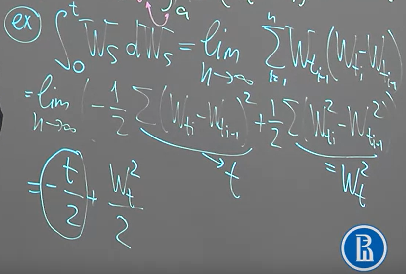
Quiz 第七題有計算這個 stochastic integral 產生的 process 之 mean and variance
這段課程的結語, 使用定義的方式來計算出 Wiener integral of process in $L_{ad}^2$ 很多時候仍然很困難
但接下來要介紹的 Ito formula 可以幫助我們計算大部分的情況
Week 7.6: Integrals of the type $∫ X_t dY_t$, where $Y_t$ is an Itô process
[Ito Process Def]:
Let $\mathcal{F}_t$ is a filtration, $b_t,\sigma_t$ are processes $\mathcal{F}_t$-adapted, $W_t$ is $\mathcal{F}_t$ Brownian motion
and $H_0$ is a random variable which is a measurable function w.r.t. $\mathcal{F}_0$
$H_t$ is a Ito process:
$H_t=H_0+\int_0^t b_sds + \int_0^t\sigma_sdW_s$
or equivalently
$dH_t=b_tdt+\sigma_tdW_t$
$H_t$ 的變化 (也還是一個 random process) 等於 $b_t$ 乘上時間的變化 $dt$, 再加上 $\sigma_t$ 乘上 Brownian motion 的變化 $dW_t$
[Stochastic Integral with Ito Process]:
Let $\mathcal{F}_t$ be some filtration, $X_t$ is $\mathcal{F}_t$-adapted and $H_t$ is a Ito process which is also $\mathcal{F}_t$-adapted.
If $X_t$ fulfilled
$\int_a^b|X_sb_s|+X_s^2\sigma_s^2ds<\infty$
then the integral is defined as
$\int_a^b X_tdH_t:=\int_a^bb_sX_xds + \int_a^b\sigma_sX_sdW_s$
r.h.s. 的第一項和第二項 integrals 之前都討論過
[Ito Lemma or Ito Formula]:
Let $H_t$ is a Ito process, i.e.
$dH_t=b_tdt+\sigma_tdW_t$
where $b_t,\sigma_t$ are processes $\mathcal{F}_t$-adapted, $W_t$ is $\mathcal{F}_t$ Brownian motion.
If $f(t,x)$ is twice continuously differentiable, then $f(t,H_t)$ be a Ito process with the following equation:
$$\color{orange}{
f(t,H_t)=f(0,H_0)+\int_0^tf_1'(s,H_s)ds + \int_0^tf_2'(s,H_s)dH_s + \frac{1}{2}\int_0^tf_{22}''(s,H_s)\sigma_s^2ds
}$$
where
$$f_1'(t,x)=\frac{\partial}{\partial t}f(t,x) \\
f_2'(t,x)=\frac{\partial}{\partial x}f(t,x) \\
f_{22}''(t,x)=\frac{\partial^2}{\partial t\partial t}f(t,x)$$
or equivalently,
$$\color{orange}{
df(t,H_t)=f_1'(t,H_t)dt + f_2'(t,H_t)dH_t + \frac{1}{2}f_{22}''(t,H_t)\sigma_t^2dt
}$$
Week 7.7: Itô’s formula
若 $H_t$ 為 Ito-process, i.e.: $b_t,\sigma_t$ are processes $\mathcal{F}_t$-adapted, $W_t$ is $\mathcal{F}_t$ Brownian motion.
$dH_t=b_tdt+\sigma_tdW_t$
If $f(t,x)$ is twice continuously differentiable, then $f(t,H_t)$ be a Ito process with the following equation:
$$f(t,H_t)\\
=f(0,H_0)+\int_0^tf_1'(s,H_s)ds + \int_0^tf_2'(s,H_s)dH_s + \frac{1}{2}\int_0^tf_{22}''(s,H_s)\sigma_s^2ds$$
Ito formula 可以用來幫助計算以下形式的積分, 假設 $g(t,x)$ is twice continuously differentiable:
$\int_0^t g(s,W_s)dW_s$
對照 Ito formula
我們在 Week 7.5 有利用 Wiener process Integral 的定義來計算過 $\int W_sdW_s$, 此時 $g(s,W_s)=W_s$, 但如果 $g(.,.)$ 複雜一點就會很難計算. 不過我們可以借用 Ito formula 來幫忙
我們令 $f$-antiderivative of $g$ w.r.t. 2nd-argument, i.e., $f_2’=g$, 注意到 $f(t,x)$ 如果加上 $h(t)$ 也滿足 $f_2’=g$, 且不影響以下推導, 可自行帶入多了一個 $h(t)$ 會發現不影響結果
由於 Brownian motion 也是 Ito process, 所以此時 $H_t=W_t$ and $\sigma_s=1$, 重新改寫 Ito formula 變成:
$f(t,W_t)=f(0,0)+\int_0^tf_1'(s,W_s)ds + \int_0^t g(s,W_s)dW_s + \frac{1}{2}\int_0^t g_2'(s,W_s)ds$
移項一下:
$$\color{orange}{
\int_0^t g(s,W_s)dW_s=f(t,W_t)-f(0,0) - \int_0^t\left(
f_1'(s,W_s)+\frac{1}{2}g_2'(s,W_s)
\right)ds
}\ldots(\square)$$
[Example]:
計算 $\int_0^t W_sdW_s$
[Sol]:
$g(t,x)=x$, 所以 $f(t,x)=\frac{1}{2}x^2$. 利用 $(\square)$ 則
$\int_0^t W_sdW_s = \frac{1}{2}W_t^2-\int_0^t\frac{1}{2}ds=\frac{1}{2}W_t^2-\frac{1}{2}t$
[Example]:
計算 $\int_0^t \frac{W_s}{1+W_s^2}dW_s$
[Sol]:
Week 7.8: Calculation of stochastic integrals using the Itô formula. Black-Scholes model
重複一次 Ito formula (in derivative form)
$df(t,H_t)=f_1'(t,H_t)dt + f_2'(t,H_t)dH_t + \frac{1}{2}f_{22}''(t,H_t)\sigma_t^2dt$
其中 $H_t$ 為 Ito-process
$dH_t=b_tdt+\sigma_tdW_t$
[Black-Scholes model Def]:
$X_t$ 為以下 Stochastic Differential Equation (SDE) 的解:
$dX_t = X_t\mu dt+X_t\sigma dW_t$
where $\mu,\sigma\in\mathbb{R},\sigma>0$, $W_t$ is $\mathcal{F}_t$ Brownian motion.
對比 Ito-process 的定義會發現 $X_t$ 是 Ito-process
上式等同於
$X_t=X_0+\mu\int_0^t X_sds+\sigma\int_0^tX_sdW_s$
證明其解為:
$X_t=X_0\cdot\exp\left\{(\mu-\frac{\sigma^2}{2})t+\sigma W_t\right\}$
[Proof]:
Let $f(t,x)=\ln x$, $H_t=X_t$ 並代入 Ito formula:
課程教授說這常用在 modeling stock prices
Week 7.9: Vasicek model. Application of the Itô formula to stochastic modelling
重複一次 Ito formula (in derivative)
$df(t,H_t)=f_1'(t,H_t)dt + f_2'(t,H_t)dH_t + \frac{1}{2}f_{22}''(t,H_t)\sigma_t^2dt$
其中 $H_t$ 為 Ito-process
$dH_t=b_tdt+\sigma_tdW_t$
[Vasicek model Def]:
$X_t$ 為以下 Stochastic Differential Equation (SDE) 的解:
$dX_t=(a-bX_t)dt+cdW_t,\qquad b,c>0$
對比 Ito-process 的定義會發現 $X_t$ 是 Ito-process
證明其解為:
$X_t=e^{-bt}X_0 + \frac{a}{b}(1-e^{-bt})+c\int_0^te^{b(s-t)}dW_s$
[Proof]:
使用 Ito formula, 並定義 $H_t=X_t$, and $f(t,x)=xe^{bt}$
得到
$$d\left(X_te^{bt}\right)=bX_te^{bt}dt+e^{bt}\left((a-bX_t)dt+cdW_t\right) \\
= ae^{bt}dt+ce^{bt}dW_t$$
所以
$X_t=e^{-bt}X_0 + \frac{a}{b}(1-e^{-bt})+c\int_0^te^{b(s-t)}dW_s$
SDE 改寫成
$dX_t=b\left(\frac{a}{b}-X_t\right)dt+cdW_t,\qquad b,c>0$
如果 $X_t>a/b$, $dX_t<0$, 也就是說 $X_t$ 的斜率為負, $X_t$ 會變小. 反之斜率為正, 值變大. 所以觀察 trajectory 為下圖:
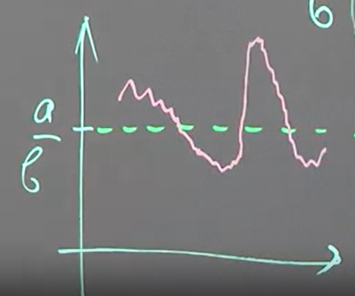
$b$ 稱為 speed of reversion
Week 7.10: Ornstein-Uhlenbeck process. Application of the Itô formula to stochastic modelling.
繼續重複 Ito formula (in derivative)
$df(t,H_t)=f_1'(t,H_t)dt + f_2'(t,H_t)dH_t + \frac{1}{2}f_{22}''(t,H_t)\sigma_t^2dt$
其中 $H_t$ 為 Ito-process
$dH_t=b_tdt+\sigma_tdW_t$
[Ornstein-Uhlenbeck process Def]:
$V_t$ 為以下 Stochastic Differential Equation (SDE) 的解:
$mdV_t=dW_t-\lambda\cdot V_tdt$
where $m$ is mass (質量), $V_t$ 表示速度, $W_t$ is Brownian motion. $\lambda$ is called friction coefficient
證明其解為:
$$V_t=e^{-\frac{\lambda}{m}t} \left(
V_0+\frac{1}{m}\int_0^t e^{\frac{\lambda}{m}s}dW_s
\right)$$
[Proof]:
使用 Ito formula, 並定義 $H_t=X_t$, and
$f(t,x)=xe^{\frac{\lambda}{m}t}$
則解為
$$V_t=e^{-\frac{\lambda}{m}t} \left(
V_0+\frac{1}{m}\int_0^t e^{\frac{\lambda}{m}s}dW_s
\right)$$
如果
$V_0\sim\mathcal{N}\left(0,\frac{1}{2\lambda m}\right) \perp W_t$
then $V_t$ is a Gaussian process with $m(t)=0$
$K(t,s)=\frac{m}{2\lambda}e^{-\frac{\lambda}{m}|t-s|}$
且看的出只與 $t-s$ 有關, 因此 auto-covariance 存在 $\gamma(t-s)=K(t,s)$
因此是 WSS, 加上是 Gaussian process, 所以也是 strictly stationary