Coursera Stochastic Processes 課程筆記, 共十篇:
- Week 0: 一些預備知識
- Week 1: Introduction & Renewal processes
- Week 2: Poisson Processes
- Week3: Markov Chains
- Week 4: Gaussian Processes
- Week 5: Stationarity and Linear filters
- Week 6: Ergodicity, differentiability, continuity
- Week 7: Stochastic integration & Itô formula
- Week 8: Lévy processes (本文)
- 整理隨機過程的連續性、微分、積分和Brownian Motion
Week 8.1: Definition of a Lévy process. Stochastic continuity and càdlàg paths
$N_t,W_t,L_t$ 分別表示 Poisson process, Brownian motion, and Levy process
$$\begin{array}{|c | c |c |}
\hline N_t & W_t & L_t \\
\hline N_0=0\text{ a.s.} & W_0=0\text{ a.s.} & L_0=0\text{ a.s.} \\
\hline \text{indep. increments} & \text{indep. increments} & \text{indep. increments} \\
\hline \text{stationary increments} & \text{stationary increments} & \text{stationary increments} \\
\hline N_t-N_s\sim Pois(\lambda(t-s)) & W_t-W_s\sim\mathcal{N}(0,t-s) & {L_t-L_s\sim\mathcal{P}(t-s),\mathcal{P}\text{ is }\color{orange}{idd}} \\
\hline
\end{array}$$
- Independent increments:
$\forall t_0<t_1<\ldots<t_n$, we have the following random variables jointly independent (所以一定也是 pairwise indep.)
$X_{t_n}-X_{t_{n-1}},\ldots,X_1-X_0$
- Stationary increments:
$\forall t,s\geq0$, and $h>0$, we have
$X_{t+h}-X_{s+h} =^d X_t-X_s$
注意到是 in distribution sense (最 weak 的那個 sense)
我們知道 “almost surely”, “in probability”, or “in mean square” senses 都會導致 in distribution sense.
- $iid$ stands for Infinitely divisible distribution: will be discussed in next section
注意到對所有的 Levy process $L_t$, 其 covariance function 有如下關係:
$$K(t,s)=Cov(L_t,L_s)\\
\text{assume } t>s \text{ } =Cov(L_t-L_s+L_s,L_s) = Cov(L_t-L_s,L_s) + Var(L_s) = Var(L_s)\\
\therefore K(t,s)=Var(L_{\min(t,s)})$$
[Cadlag Function Def]:
中文稱 “右連左極函數”
We say $f$ is a Cadlag function, if 左右 limit 都存在且定義 $f$ 為右 limit 的值
$$\exists\lim_{s\rightarrow t,s<t} f(s) =: f(t^-) \\
\exists\lim_{s\rightarrow t,s>t} f(s) =: f(t^+) = f(t)$$
Wiki 的介紹很清楚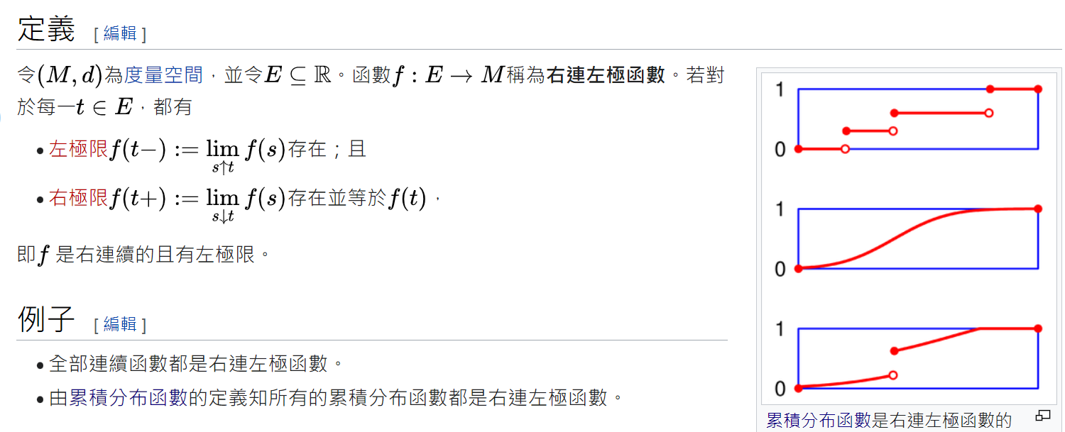
記得在 Brownian motion 時有講到 Kolmogorov continuity theorem: 一定存在一個 continuous modification of a Brownian motion 類似.
所以看到 Brownian motion 可以只考慮其 almost surely continuous trajectories 的版本
[Proposition, Cadlag Trajectories of Levy Process]:
在 Levy process 也有類似的情況. 給定一個 Levy process $L_t$
存在另一個 process $L_t’$ such that 所有 trajectories 都是 almost surely Cadlag function.
Week 8.2: Examples of Lévy processes. Calculation of the characteristic function in particular cases
[Infinitely Divisible Distributions Def]:
$\xi$ is a infinitely divisible distribution if $\forall n\geq2$, $\exists Y_1,\ldots,Y_n$ - i.i.d. such that
$\xi=^d Y_1+\dots+Y_n$
Note that it is equals in distribution sense. It is equivalent to saying:
$$\Phi_\xi(u)=\left(\Phi_{Y_1}(u)\right)^n, \qquad \forall n \\
\Longleftrightarrow \left(\Phi_\xi(u)\right)^{1/n} \text{ is a characteristic function}, \qquad\forall n$$
where $\Phi_\xi(u)$ is the characteristic function of random variable $\xi$
[Levy Process can be Characterized by an I.D.D.]:
1. $\forall$ Levy process $L_t$ at $\forall$ time $t^*$, $L_{t^*}$ has an infinitely divisible distribution
2. $\forall$ infinitely divisible distribution, $\exists$ a Levy process $L_t$ such that $L_1$ has this distribution
[Proof]:
只證明第一條. $L_t$ 可以改寫如下: $\forall n$ 都滿足
$L_t=\sum_{k=1}^n\left(L_{t\cdot\frac{k}{n}} - L_{t\cdot\frac{k-1}{n}}\right)$
由於 stationary increments 特性
$\left(L_{t\cdot\frac{k}{n}} - L_{t\cdot\frac{k-1}{n}} \right) =^d L_{\frac{t}{n}}$
再由於 independent increments 特性, 變成 $n$ 個 i.i.d. random variables 相加. Q.E.D.
[Normal Distribution is an i.d.d.]: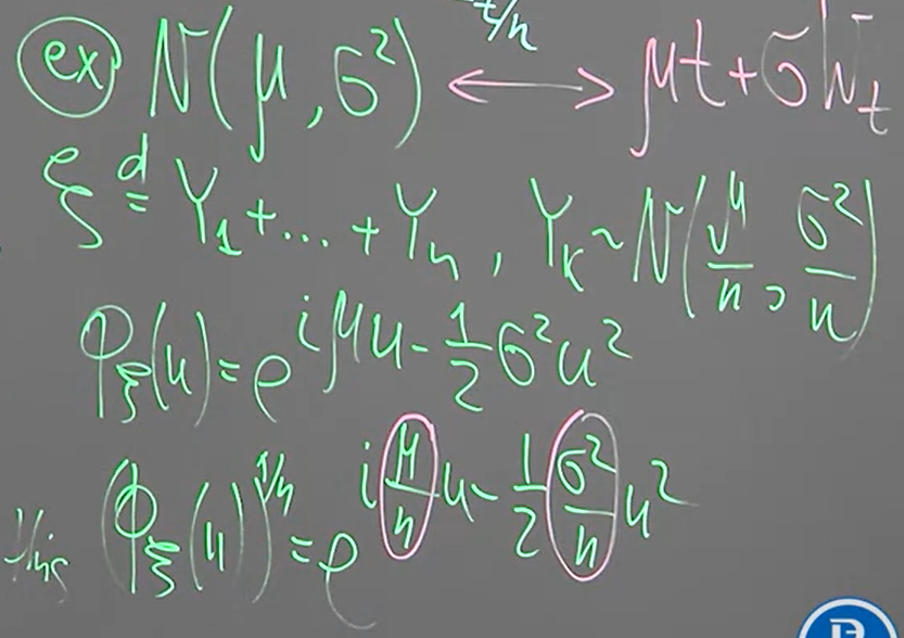
所以可以發現 $L_t$ is a Levy process ($W_t$ is a Brownian motion)
$L_t=\mu t+\sigma W_t$; 且 $L_1\sim\mathcal{N}(\mu,\sigma^2)$
[Cauchy Distribution is an i.d.d.]:
Cauchy distribution 的 p.d.f. 為:
$p(x)=\frac{1}{\pi\gamma\left[1+\left(\frac{x-x_0}{\gamma}\right)^2\right]}$
其中 $x_0$ 稱為 location parameter, $\gamma$ 稱為 scale parameter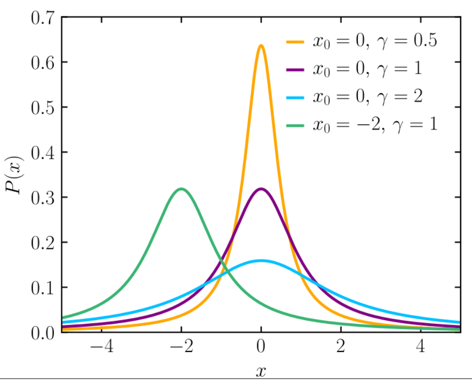
觀察特徵函數可以發現是 i.d.d.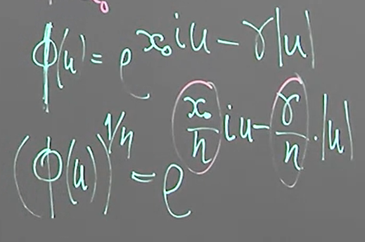
[Gamma Distribution is an i.d.d.]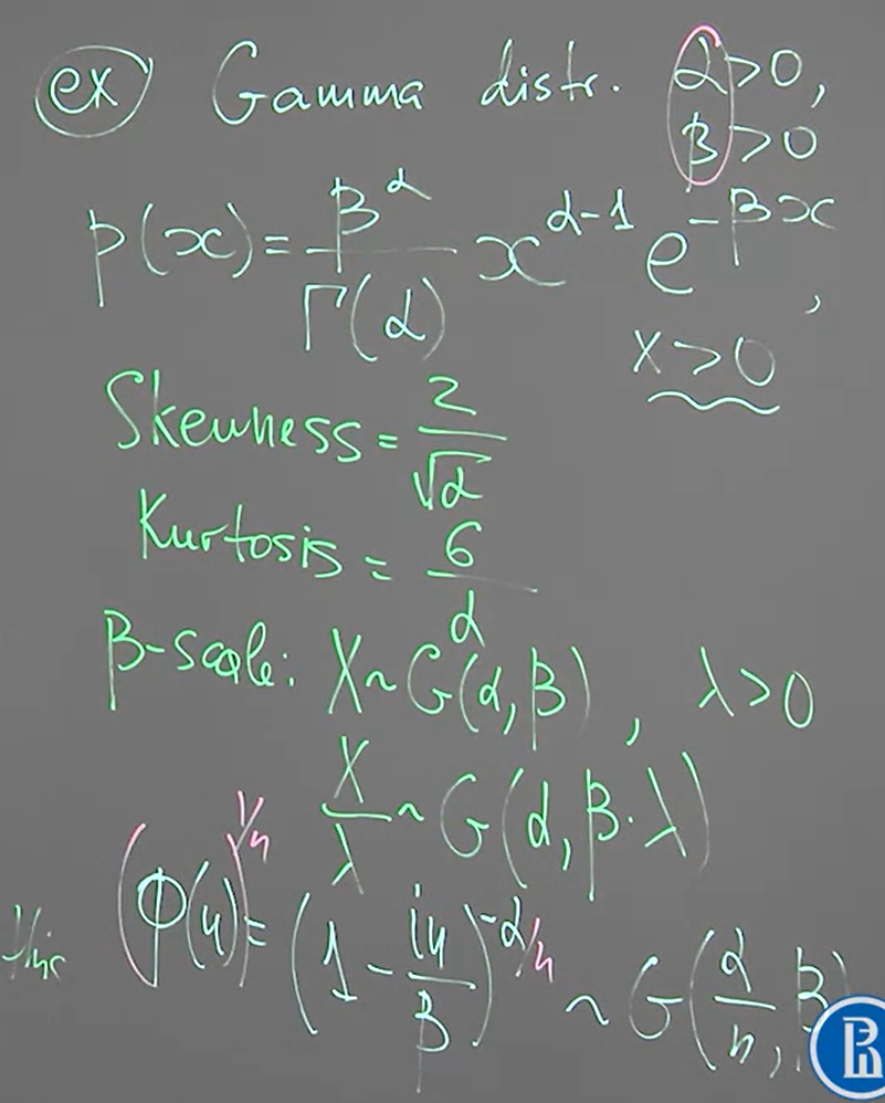
Distributions that are infinitely divisible distributions: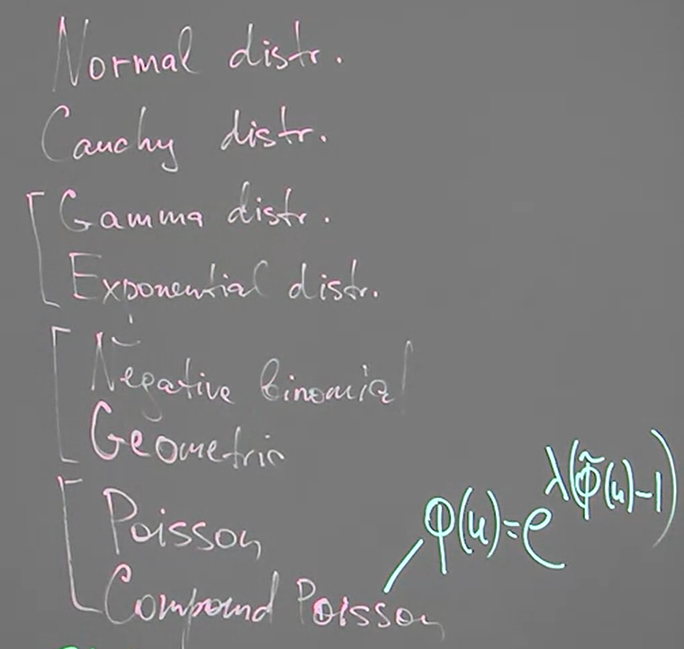
[Stable Distribution Def]:
We say that $\xi$ is stable distribution if $\forall n\geq2$, $\exists$ $a_n>0,b_n\in\mathbb{R}$
$\xi,\xi_1,\ldots,\xi_n$ - are i.i.d. such that
$\xi_1+\ldots+\xi_n =^d a_n\xi+b_n$
是 stable distribution 一定是 infinitely divisible, 很容易看出來, 只要改寫成
$\left(\frac{\xi_1}{a_n}-\frac{b_n}{n\cdot a_n}\right) + \ldots + \left(\frac{\xi_n}{a_n}-\frac{b_n}{n\cdot a_n}\right) =^d \xi$
反之不成立
所以上述的 i.d.d. 中, 只有 Normal and Cauch distributions 是 stable
Week 8.3: Relation to the infinitely divisible distributions
[Properties of Infinitely Divisible Distributions]:
Let $\xi$ is a i.d.d. then
1. $\Phi_\xi(u)=0$ doesn’t have any $\mathbb{R}$ solution
i.e. all solutions are imaginary numbers. 特徵方程式的 roots 沒有實數解
2. Support set of $\xi$, $Supp(\xi)$, is unbounded
Random variable $\xi$ 為一個 measurable function $\Omega\rightarrow\mathbb{R}$. 而 support of a measurable function $\mu$ 定義為:
$Supp(\mu):=\left\{x:\forall\text{ open set }G\text{ containing }x\text{ s.t. }\mu(G)>0\right\}$
參考 wiki 的定義):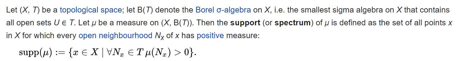
白話是任何 $x$ 的 open neighbourhood 的 measure 都 $>0$, 則 $x$ 屬於 support set
因此 random variable 的 support set 就用 measurable function 的方式去想
[Uniform Distribution is NOT i.d.d.]:
Let $\xi$ is uniform distribution $\mathcal{U}(a,b)$, then the characteristic function is
$\Phi_\xi(u)=\int_a^b e^{iux}\frac{1}{b-a}dx=\frac{1}{b-a}\cdot\frac{e^{iua}}{iu}\cdot\left(e^{iu(b-a)}-1\right)$
We have $\Phi_\xi(u)=0$ if and only if
$e^{iu(b-a)}=1 \Longleftrightarrow u=\frac{2\pi k}{b-a},\qquad k\in\mathbb{Z}/\{0\}$
所以存在 $\mathbb{R}$ 的 root, 因此不是 infinitely divisible distributions
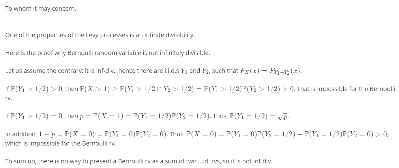
[Bernoulli Distribution is NOT i.d.d.]:
Let $\xi$ is Bernoulli random variable
$$\xi=\left\{
\begin{array}{rl}
1, & p\\
0, & 1-p
\end{array}
\right.$$
then $Supp(\xi)=\{0,1\}$, so is not bounded and hence NOT infinitely divisible distributions
我們常看到的 distribution 大部分都是 infinitely divisible distribution, 如
Gaussian, Cauchy, Gamma, Poisson, Compound Poisson
但是 uniform and Bernoulli distributions 不是 i.d.d.
最後試題計算一下 binomial distribution $Bin(n,p)$ 的特徵函數:
$$\Phi_X(u)=\mathbb{E}\left[e^{iuX}\right]=\sum_{k=0}^n e^{iuk}\mathcal{P}(X=k) \\
= \sum_{k=0}^n e^{iuk}\frac{n!}{k!(n-k)!}p^k(1-p)^{n-k} \\
= \sum_{k=0}^n\frac{n!}{k!(n-k)!}(e^{iu}p)^k(1-p)^{n-k} = (e^{iu}p+(1-p))^n$$
Week 8.4: Characteristic exponent
[Characteristic Exponent Def with Proposition]:
$\forall$ Levy process $L_t$, $\exists \Psi:\mathbb{R}\rightarrow\mathbb{C}$ call characteristic exponent, such that
$\Phi_{L_t}(u)=\mathbb{E}[e^{iuL_t}]=e^{t\cdot\Psi(u)}$
[Example 1]:
$L_t=\mu\cdot t$, 其 characteristic function is $\Phi_{L_t}(u)=\mathbb{E}[e^{iu\mu t}]$, 所以 $\Psi(u)=iu\mu$
[Brownian Motion Example 2]:
$L_t=\sigma W_t$, where $W_t$ is a Brownian motion. 所以 $L_t\sim\mathcal{N}(0,\sigma^2t)$.
我們知道 $X\sim\mathcal{N}(\mu,\sigma^2)$ 的特徵方程式為:
$\Phi_X(u)=e^{i\mu u-\frac{1}{2}\sigma^2u^2}$
所以
$\Phi_{L_t}(u)=e^{-\frac{1}{2}\sigma^2t u^2}\Longrightarrow \Psi(u)=-\frac{1}{2}\sigma^2u^2$
[Compound Poisson processes Example 3]:
Let $X_t$ is a Compound Poisson processes. We have it’s characteristic function of increments as:
$\Phi_{X_t-X_s}(u)=e^{\lambda(t-s)(\Phi_{\xi_1}(u)-1)}$
Therefore, characteristic function of $L_t=X_t$:
$\Phi_{L_t}(u)=e^{\lambda t(\Phi_{\xi_1}(u)-1)}$
and hence
$$\Psi(u)=\lambda(\Phi_{\xi_1}(u)-1) \\
=\lambda\left( \int e^{iux}\mathcal{P}_{\xi_1}(x)dx - \int\mathcal{P}_{\xi_1}(x)dx \right) \\
= \int (e^{iux}-1)\lambda \mathcal{P}_{\xi_1}(x)dx
=\int (e^{iux}-1)\lambda F_{\xi_1}(dx)$$
[Linear Brownian Motion Plus Compound Poisson processes Example 4]:
Let $L_t$ is
$L_t=\mu t+\sigma W_t + C.P.P.$
then we have
$\Psi(u)=iu\mu-\frac{1}{2}\sigma^2u^2 + \int (e^{iux}-1)\lambda F_\xi(dx)$
這個形式很重要, for such Levy process, 其特徵方程式可以 explicitly 寫出來
[Corollaries]:
1. The distribution of $L_t$ is determined by $L_1$
$\Phi_{L_1}(u)=e^{\Psi(u)}$
所以可以由 $L_1$ 決定出 characteristic exponent $\Psi(u)$
而知道 $\Psi(u)$ 我們就知道任何時間點的 characteristic function, 也就決定了 distribution
2. Expectation and variance of $L_t$
$$\mathbb{E}L_t=t\cdot\mathbb{E}L_1 \\
Var(L_t)=t\cdot Var(L_1) \\
K(t,s) =Var(L_{\min(t,s)}) = \min(t,s)\cdot Var(L_1)$$
由此 $K(t,s)$ 可知, Levy process is NOT stationary (in any sense). 因為 WSS 必須滿足 $K(t,s)=K(t+h,s+h)$, 然而 $\min(t,s)\neq \min(t+h,s+h)$
注意到, Levy process is NOT stationary but is stationary increment
Week 8.5: Properties of a Lévy process, which directly follow from the existence of characteristic exponent
[Levy Measure Def]:
Levy measure of a Levy process $X_t$ is defined as
$$\nu(B)=\mathbb{E}\left[
\# t\in[0,1]: \triangle X_t \in B
\right], \qquad \forall B\subset\mathbb{R} \setminus\{0\}$$
where $\triangle X_t=X_t-X_{t^-}$ (size of jump), also reference to definition of Cadlag function
$B$ 定義了我們要關注的那些 jump 值, 而 measure 就是: 有多少 (以期望值來看) random variables 他們的 jump 值屬於 $B$, 且 random variables 只限制在 $t\in[0,1]$
又或者這麼說, 對於 $X_t,\forall t\in[0,1]$ 這些 random variables 來說, measure 就是發生 jump 次數的期望值 (constrained on jump 的值是我們要的, i.e. in $B$)
此段課程後面會提供一個 Levy measure 的充要條件, 實在很神奇
這定義是否符合 measure 之定義? 檢查如下特性
1. Non-negativity: $\nu(B)\geq 0$
2. Null empty set: $\nu(\phi) = 0$
3. Countable additivity:
For all countable collections ${B_k}$ of pairwise disjoint sets
$\nu\left(\bigcup_{k=1}^\infty B_k \right) = \bigcup_{k=1}^\infty \nu(B_k)$
可發現 $\nu$ 符合 measure 定義, 所以是個 measure
Brownain motion is continuous a.e. 所以 $\nu(B)=0$
Poisson process 如圖所示
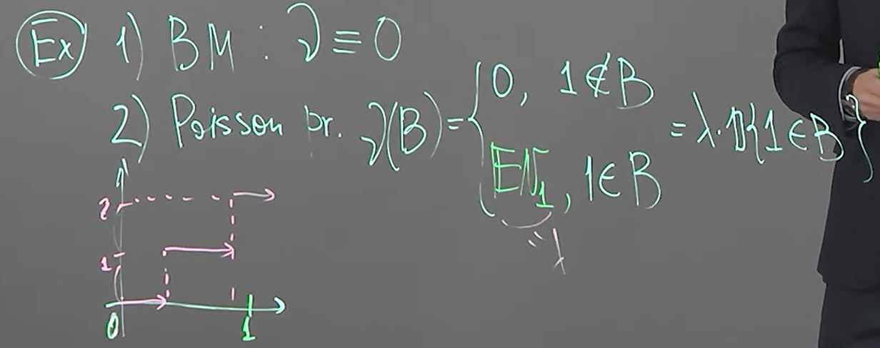
考慮 Compound Poisson process, let $N_t$ is Poisson process, and $\xi_1,\xi_2,…$ are i.i.d. then C.P.P. $X_t$ is defined as
$X_t=\sum_{k=1}^{N_t} \xi_k$
其 Levy measure 如下:
$$\nu(B)=\lambda\cdot\mathcal{P}(\xi_1\in B) \\
= \int_B \lambda \mathcal{P}_\xi(x)dx := \int_B s(x)dx$$
where $s(x)$ is called Levy density
$s(x):=\lambda \mathcal{P}_\xi(x)$
and we have $\nu(dx)=s(x)dx$
可以這麼想, 在原來的 Poisson process, 每一次的 jump 都固定是 $1$, 但在 C.P.P. jump 的值是根據 $\xi_k$ 來決定的. 所以能不能算進一次 jump 要看 jump 的值是不是在 $B$ 中
[Sufficient and Necessary Condition of Levy Measure]:
If $\nu$ is a Levy measure for some Levy process $L_t$, if and only if satisfying
$$\int_{|x|<1} x^2\nu(dx) =\int_{|x|<1} x^2s(x)dx<\infty \\
\int_{|x|\geq1} \nu(dx)=\int_{|x|\geq1} s(x)dx<\infty$$
Week 8.6: Lévy-Khintchine representation and Lévy-Khintchine triplet-1
💡 課程老師說這是整個課程最重要的定理
[Levy-Khintchine Theorem]:
The characteristic exponent $\Psi(u)$ of a Levy process $L_t$ can be represented as follows:
$$\color{orange}{
\Psi(u)=iu\mu-\frac{1}{2}u^2\sigma^2 + \int_{\mathbb{R}}\left(
e^{iux}-1-iux\cdot\mathbf{1}\{|x|<1\}
\right)\nu(dx)
}$$
where $\mu\in\mathbb{R},\sigma\geq0$, and $\nu$ is a Levy measure. $(\mu,\sigma,\nu)$ is called Levy triplet
which completely determined the distribution of Levy process at any time moment $t$
可以證明 $\forall L_t$ - Levy process, 可以表示如下
$X_t = \underbrace{\mu t + \sigma W_t}_\text{continuous part} + \underbrace{\mathcal{J}_t}_{\text{jump part}}$
所以 Levy process 的 continuous part 可以視為 Brownian motion
而 jump part $\mathcal{J}_t$:
$$\mathcal{J}_t \approx
\overbrace{
\left(
\sum_{0<s<t,|\triangle X_s|>1} \triangle X_s
\right)
}^{\text{C.P.P.}}
+
\left(
\lim_{\varepsilon\rightarrow0}
\overbrace{
\sum_{0<s<t,\varepsilon<|\triangle X_s|\leq1} \triangle X_s
}^{\text{C.P.P.}}
\right)$$
我們可以將 Levy process 的 trajectory 畫出來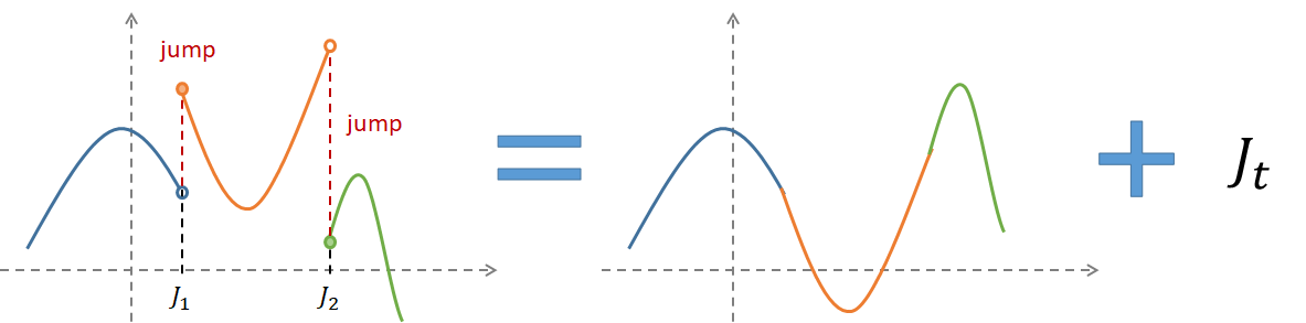
trajectory_of_Levy_process.pptx
接下來下一節課程會介紹一個 sufficient condition 使我們可以把 jump process 的 limit 那段拿掉, 使得 jump process 完全可以由一個 C.P.P. 替代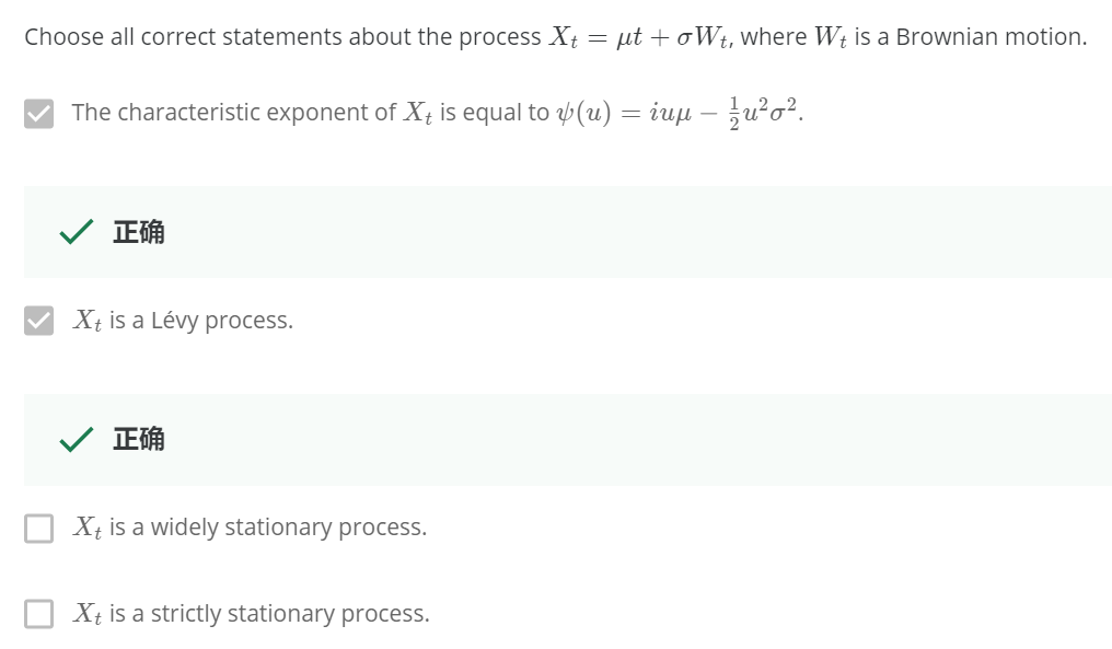
Week 8.7: Lévy-Khintchine representation and Lévy-Khintchine triplet-2
重複一次 Levy process 的 characteristic exponent:
$$\Psi(u)=iu\mu-\frac{1}{2}u^2\sigma^2 + \int_{\mathbb{R}}\left(
e^{iux}-1-
\color{orange}{
iux\cdot\mathbf{1}\{|x|<1\}
}
\right)\nu(dx)$$
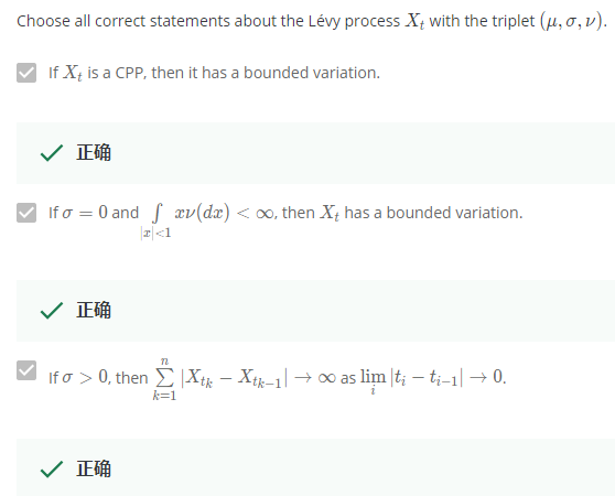
有些情況下可以簡化上式, 尤其橘色部分. 首先回顧一下什麼是 bounded variation
[Bounded Variation of a Stochastic Processes]:
對於一個 process $X_t$, 考慮一個 partition $\bigtriangleup:0=t_0<t_1<...<t_n=t$
如果滿足以下條件, 則稱 $X_t$ is bounded variation:
$\lim_{|\bigtriangleup|\rightarrow0} \sum_{k=1}^n | X_{t_k}-X_{t_{k-1}} | < \infty$
$|\bigtriangleup|\rightarrow0$ 表示:
$\max_{k=0,...,n}\{|t_k-t_{k-1}|\}\rightarrow0, \text{ for }n\rightarrow0$
注意到 Brownian motion $W_t$ 不是 bounded variation
[When Levy Process is Bounded Variation]:
一個 Levy process $L_t$ 是 bounded variation 若且為若
$$\begin{align}
\sigma=0 \\
\int_{|x|<1} x\nu(dx) < \infty
\end{align}$$
條件 $(2)$ 會有如下結果
$\int_\mathbb{R}iux\cdot\mathbf{1}\{|x|<1\}\nu(dx) = iu\int_{|x|<1}x\nu(dx)<\infty$
因此 characteristic exponent 變成:
$$\Psi(u)=iu\mu-\frac{1}{2}u^2\sigma^2 + \int_{\mathbb{R}}\left(
e^{iux}-1-
iux\cdot\mathbf{1}\{|x|<1\}
\right)\nu(dx) \\
=iu\mu +
\int_{\mathbb{R}}(e^{iux}-1)\nu(dx)-iu\int_{|x|<1}x\nu(dx) \\
= iu\left(\mu-\int_{|x|<1}x\nu(dx)\right) + \int_{\mathbb{R}}(e^{iux}-1)\nu(dx)$$
所以 characteristic function: $\Phi(u)=\exp\{t\cdot\Psi(u)\}$
重寫一遍, 這很重要
$$\color{orange}{
\Psi(u) = iu
\underbrace{\left(\mu-\int_{|x|<1}x\nu(dx)\right)}_{=\tilde{\mu}}
+ \int_{\mathbb{R}}(e^{iux}-1)\nu(dx)
}$$
or
$$\color{orange}{
\Psi(u) = iu
\underbrace{\left(\mu-\int_{|x|<1}x\cdot s(x)dx\right)}_{\tilde{\mu}}
+ \int_{\mathbb{R}}(e^{iux}-1)\cdot s(x)dx
}$$
where $s(x)$ is Levy density
[When Levy Process is C.P.P.]
一個 Levy process $L_t$ 是 C.P.P. 若且為若
$$\begin{align}
\sigma=0, \\
\int_{\mathbb{R}}\nu(dx)=\nu(\mathbb{R})<\infty
\end{align}$$
可以發現這樣的 $L_t$ 也是 bounded variation, 所以也可以簡化
[When Levy Process is Subordinator]:
一個 Levy process $L_t$ 稱為 subordinator 如果滿足
$$\begin{align}
X_t\geq0\text{ a.s. }\Longleftrightarrow X_t\geq X_s\text{ a.s. }, \forall t\geq s
\end{align}$$
上式會等價是因為 Levy process 的 stationary increment. i.e.
$X_t-X_s =^d X_{t-s}, \qquad \forall t\geq s$
而 Levy process $L_t$ 為 subordinator 若且為若
$$\begin{align}
\sigma=0 \\
\nu(\mathbb{R}^-)=0 \\
\int_0^1 x\nu(dx)<\infty
\end{align}$$
式 (7) 的 Levy measure 表示 jump 的值一定都是正的 (為負的次數其 measure 為 0)
一樣可以發現這樣的 $L_t$ 也是 bounded variation, 所以也可以簡化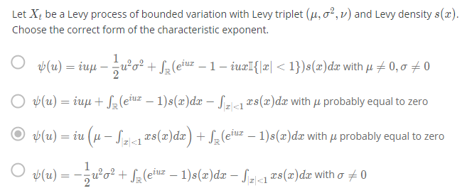
最後一個問題是因為 $\sigma>0$ 表示有 Brownian motion, 所以 variation 不會 bounded
Week 8.8: Lévy-Khintchine representation and Lévy-Khintchine triplet-3
Recap
Levy process 常用來描述 jumps, recap Levy process $L_t$
其 characteristic exponent 為
$$\Psi(u)=iu\mu-\frac{1}{2}u^2\sigma^2 + \int_{\mathbb{R}}\left(
e^{iux}-1-
iux\cdot\mathbf{1}\{|x|<1\}
\right)\nu(dx)$$
然後 characteristic function 為
$\Phi_{L_t}(u)=\exp\{t\cdot \Psi(u)\}$
而 $\nu(x)$ 是 Levy measure
$\nu(B)=\int_B s(x)dx$
稱 $s(x)$ 為 Levy density, 滿足
$$\begin{align}
\int_{|x|<1} x^2\nu(dx) =\int_{|x|<1} x^2s(x)dx<\infty \\
\int_{|x|\geq1} \nu(dx)=\int_{|x|\geq1} s(x)dx<\infty
\end{align}$$
Recap 結束
由 Levy measure and density 式子 (9) and (10) 知道, characteristic exponent 的積分項存在, 分析如下
$$\int_{\mathbb{R}}\left(
e^{iux}-1-
iux\cdot\mathbf{1}\{|x|<1\}
\right)\nu(dx) \\
= \int_{|x|<1}\left(e^{iux}-1-iux\right)\nu(dx)
+ \int_{|x|\geq1}(e^{iux}-1)\nu(dx) \\
\leq \int_{|x|<1}\left(O(x^2)\cdot u^2\right)\nu(dx) + \int_{|x|\geq1}2\nu(dx)<\infty$$
我們可以分析 $r$ 最小可以多小, 使得下式仍滿足
$\int_{|x|<1}x^r\nu(dx)<\infty$
我們知道如果 $r$ 滿足的話, 則 $\forall s
[Stable Processes Def]:
Stable processes are Levy processes which have stable distribution at any time moment.
以下照老師的說法寫下的, 不是很肯定
[Levy Process Defined by Stable Process]:
$S_t$ is a Levy process if $\forall a>0$, $\exists b:\mathbb{R}^+\rightarrow\mathbb{R}$, $\alpha\in(0,2]$, such that
$$\left\{ S_{at}\right\}_{t\geq0}
=^d
\left\{ a^{1/\alpha}S_t+b(t)\right\}_{t\geq0}$$
Brownian motion is a stable process, 因為 $\alpha=2$, $b(t)=0$ 滿足上式
$W_{at}\sim\mathcal{N}(0,at)\sim\sqrt{2}\cdot\mathcal{N}(0,t)\sim\sqrt{2}\cdot W_t$
For stable processes, $BG(\nu)=\alpha$
如果 $\alpha\approx0$, 則 trajectories 會很接近 C.P.P., 而如果 $\alpha\approx2$, 則 trajectories 會很接近 Brownian motion, 其他則介於中間的兩者混合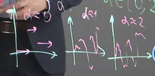
Week 8.9: Modelling of jump-type dynamics. Lévy-based models
這節主要講如何從 data 去 estimate 出對應的 Levy process
$X_t$ is a Levy process with bounded variation, 所以特徵方程式為:
$$\Phi_{X_\Delta}(u) = \exp\left\{
\Delta\cdot\left(
iu\tilde\mu+\int_\mathbb{R}(e^{iux}-1)s(x)dx
\right)
\right\}$$
對其一次和二次微分: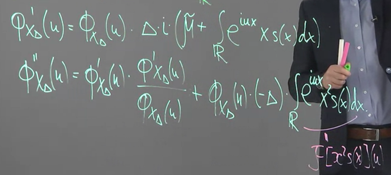
注意到二次微分跑出了一個 Fourier transform 項, 所以改寫一下變成
$$\begin{align}
\mathcal{F}[x^2s(x)](u)=\frac{-1}{\Delta}\cdot\left(
\frac{\Phi_{X_\Delta}''(u)}{\Phi_{X_\Delta}(u)} - \left(\frac{\Phi_{X_\Delta}'(u)}{\Phi_{X_\Delta}(u)}\right)^2
\right)
\end{align}$$
所以如果我們有如下的 data:
$X_\Delta,X_{2\Delta},...,X_{n\Delta}$
我們可以估計出 $\Phi$ 如下:
$$\hat{\Phi}_{X_\Delta}(u)=\frac{1}{n}\sum_{k=1}^n \exp\left\{iu\left(X_{k\Delta}-X_{(k-1)\Delta}\right)
\right\}$$
我不是很懂為何可以這麼估計, 發問題到論壇了.
因此對其微分也就得到估計的 $\hat\Phi’,\hat\Phi’’$, 然後可以得到式 (11) 的結果, 再對其求 inverse Fourier transform 可以得到 Levy density $s(x)$
老實說沒有例子很難想像怎麼做…. 🙁
Week 8.10: Time-changed stochastic processes. Monroe theorem
有始有終吧, 最後一課了!!
說明一些 Levy-based model
課程說單純的 Levy process 對於真實情況仍過於簡化, 因此要有一些變形, 其中一個例子是 stochastic time change model
[Stochastic Time Change Model]:
$X_t$ is a Levy process, 其中 $t=T(s)$, $T(s)$ 是一個 subordinator Levy process, 所以變成 $X_{T(s)}$
同時如果 $X_t\perp T(s)$ 則 $X_{T(s)}$ 也會是 Levy process
一個例子如下圖, $t$ 有時很密集, 有時很鬆散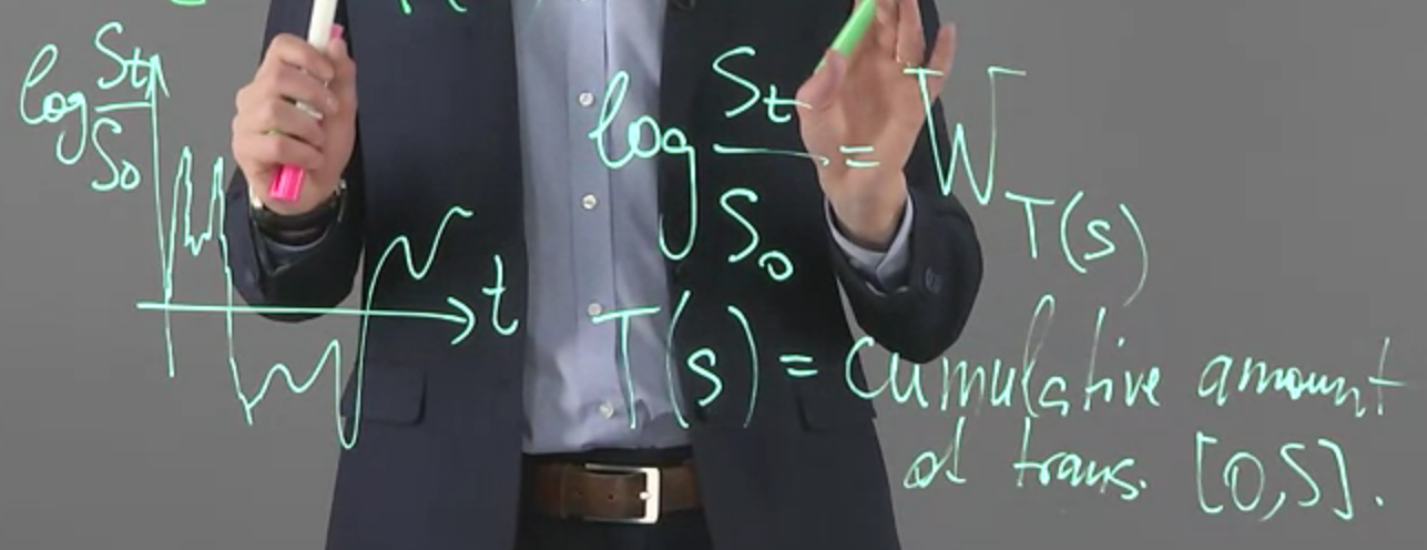
$T(s)$ 是 cumulative amount of transactions in time interval $[0,s]$
第二個例子真的聽不懂…
課程結束! 最後剩 Quiz and Final Exam! 👏