Score Function and Fisher Information Matrix

---

Bayesian statistics 視 dataset $\mathcal{D}=\{x_1,...,x_n\}$ 為固定, 而 model parameter $\theta$ 為 random variables, 透過假設 prior $p(\theta)$, 利用 Bayes rule 可得 posterior $p(\theta|\mathcal{D})$. 而估計的參數就是 posterior 的 mode, i.e. $\theta_{map}$ (Maximum A Posterior, MAP)

關於 Fisher information matrix 在 Bayesian 觀點的用途, 其中一個為幫助定義一個特殊的 prior distribution (Jeffreys prior), 使得如果 parameter $\theta$ 重新定義成 $\phi$, 例如 $\phi=f(\theta)$, 則 MAP 解不會改變. 關於這部分還請參考 Machine Learning: a Probabilistic Perspective by Kevin Patrick Murphy. Chapters 5 的 Figure 5.2 圖很清楚

反之 Frequentist statistics 視 dataset $\mathcal{D}=\{X_1,...,X_n\}$ 為 random variables, 透過真實 $\theta^*$ 採樣出 $K$ 組 datasets, 每一組 dataset $\mathcal{D}^k$ 都可以求得一個 $\theta_{mle}^k$ (MLE 表示 Maximum Likelihood Estimator), 則 $\theta_{mle}^k$ 跟 $\theta^*$ 的關係可藉由 Fisher information matrix 看出來

本文探討 score function 和 Fisher information matrix 的定義, 重點會放在怎麼直觀理解. 然後會說明 Fisher information matrix 在 Frequentist statistics 角度代表什麼意義.

先定義一波

Score Function

---

[Score Function Definition]:
 針對某一點 data point $x$, 在 $\hat{\theta}$ 點的 log-likelihood 的 gradient 定義為 score function:
 

$$\begin{align} s(x,\hat{\theta}) \triangleq \nabla_\theta \log p(x|\hat\theta) \end{align}$$

注意到如果 $x$ 是 random variables, $s(x,\hat{\theta})$ 也會是 random variable
在 Frequentist statistics 觀點下, data $x$ 是 random variables, 所以可以對 true parameter $\theta^*$ 的 data distribution $p(x|\theta^*)$ 計算期望值:

$$\begin{align} \mathbb{E}_{p(x|\theta^*)}[s(x,\hat{\theta})] = \int p(x|\theta^*) \nabla_\theta \log p(x|\hat\theta) dx \end{align}$$

我們舉個離散的例子來說明式 (2):

score_function_example.drawio

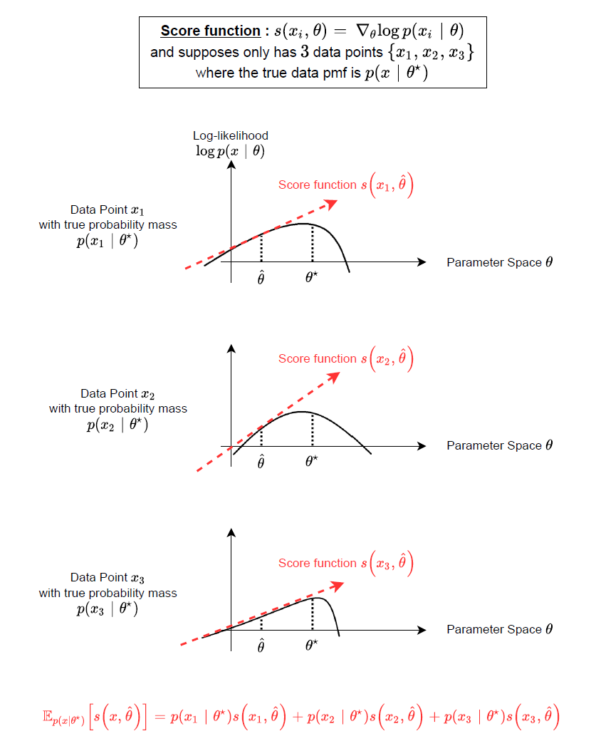
可以看到 score function 相當於在描述 parameter 變化對於 log-likelihood 的變化程度.
而該變化程度在真實 $\theta^*$ 那點的期望值為 $0$, i.e. 在 $\hat\theta=\theta^*$ 這點計算 score function 的期望值:

$$\mathbb{E}_{p(x|\theta^*)}[s(x,\theta^*)] = \int p(x|\theta^*) \nabla_\theta \log p(x|\theta^*) dx \\ = \int p(x|\theta^*)\frac{\nabla_\theta p(x|\theta^*)}{p(x|\theta^*)} dx \\ = \int \nabla_\theta p(x|\theta^*) dx \\ = \nabla_\theta \int p(x|\theta^*) dx = \nabla_\theta 1 = 0$$

💡 注意到計算期望值都是基於真實資料分佈, i.e. $p(x|\theta^*)$. 為何強調這一點, 是因為我們手頭上的 training data 一般來說都是假設從真實分佈取樣出來的, 也就是說只要用 training data 計算期望值, 隱含的假設就是用 $p(x|\theta^*)$ 來計算.

因此我們有

$$\begin{align} \mathbb{E}_{p(x|\theta^*)}[s(x,\theta^*)] = 0 \end{align}$$

💡 其實對任何其他點 $\hat{\theta}$ 式 (3) 也成立, i.e. $\mathbb{E}_{p(x|\hat{\theta})}[s(x,\hat{\theta})]=0$. 注意到期望值必須基於 $p(x|\hat\theta)$ 而非真實資料分佈了.

Fisher Information Matrix

---

💡 $\mathbb{E}_{p(x|\theta^*)}[\cdot]$ 我們簡寫為 $\mathbb{E}_{p^*}[\cdot]$

[Fisher Information Matrix Definition]:
 在 $\hat{\theta}$ 點的 Fisher information matrix 定義為:
 

$$I(\theta^* ; \hat\theta) =\mathbb{E}_{p^*}\left[ s(x,\hat\theta)s(x,\hat\theta)^T \right] \\ = \mathbb{E}_{p^*}\left[\nabla_\theta\log p(x|\hat\theta)\nabla_\theta\log p(x|\hat\theta)^T\right]$$
 其中 $\theta^*$ 為真實資料的參數
其實就是 score function 的 second moment.

Fisher information matrix 在 $\hat\theta=\theta^*$ 此點上為:

$$\begin{align} I(\theta^* ; \theta^*) =\mathbb{E}_{p^*}\left[ (s(x,\theta^*)-0)(s(x,\theta^*)-0)^T \right] \\ = \mathbb{E}_{p^*}\left[ (s(x,\theta^*)- \mathbb{E}_{p^*}[s(x,\theta^*)] )(s(x,\theta^*)- \mathbb{E}_{p^*}[s(x,\theta^*)] )^T \right] \\ = Cov_{p^*}\left( s(x,\theta^*),s(x,\theta^*) \right) \end{align}$$
由於我們已經知道 score function 在 $\hat\theta=\theta^*$ 的期望值是 $0$ , 因此 Fisher information matrix 變成 Covariance matrix of score function

💡 同樣對任何其他點 $\hat{\theta}$ 式 (6) 也成立, i.e. $I(\hat\theta ; \hat\theta)=Cov_{\hat p}(s(x,\hat\theta),s(x,\hat\theta))$. 同樣注意到期望值必須基於 $p(x|\hat\theta)$ 而非真實資料分佈了.

示意圖為:
score_function_example_on_true_parameters.drawio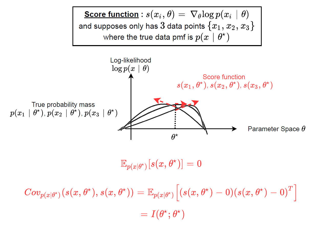

另外假如我們思考 score function (gradient) 計算的是一次微分, 可以想成是斜率. 那如果考慮二次微分 (Hseeian matrix), 則可想成是 curvature, 因此示意圖為:
Hessian_example_on_true_parameters.drawio
curvature_example.pptx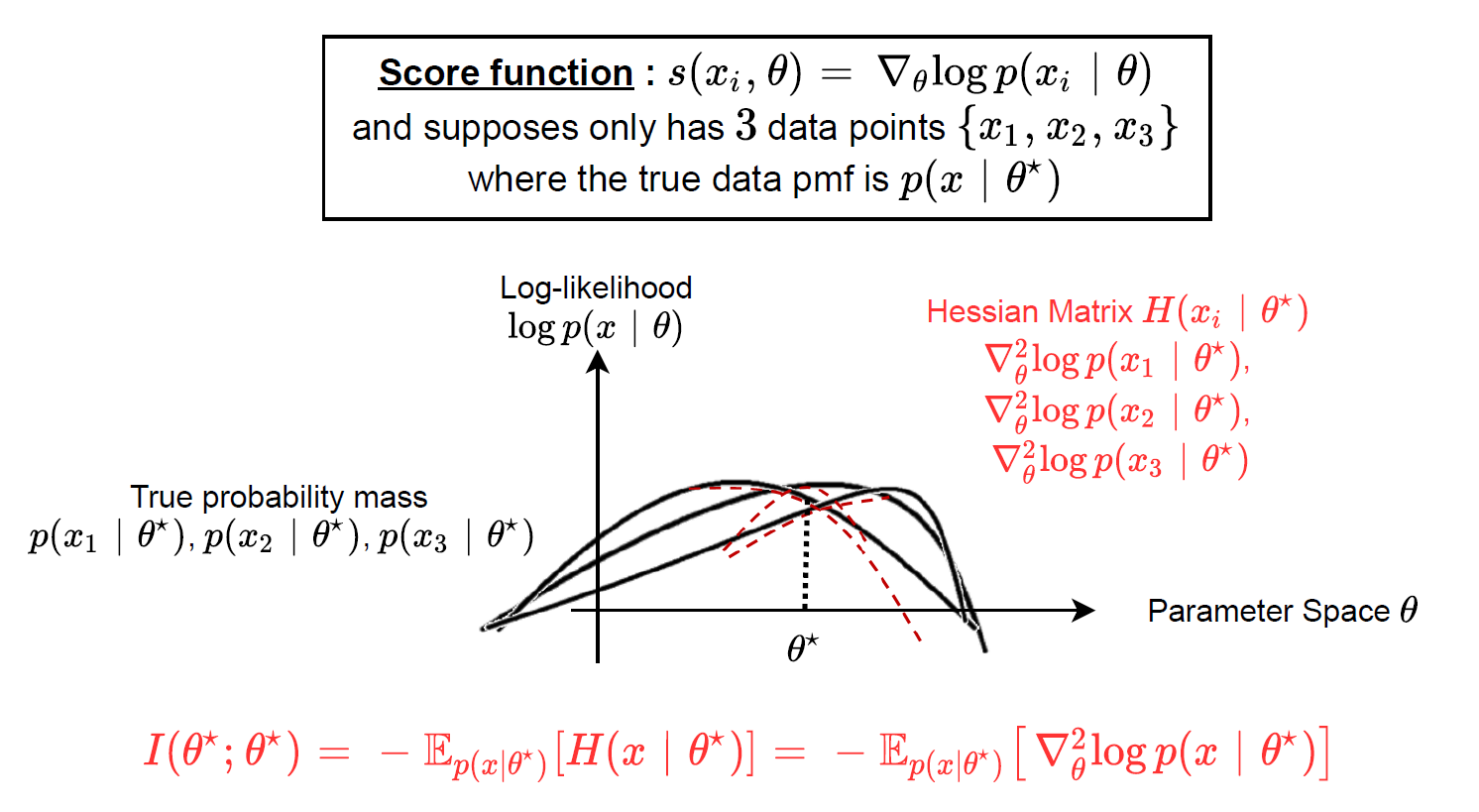

紅色的那三條 curves 就是 3 個 data points 的 Hessian matrices. 因此 Hessian matrix (at $\theta^*$) 的期望值直觀上可以想成 log-likelihood 的 graph 在 $\theta^*$ 的彎曲程度 (curvature).
以上這個觀點其實跟 Fisher information matrix 有關聯的, 描述如下:
“Fisher information matrix = score function 的 covariance matrix” 等於 “負的 Hessian matrix 之期望值”. 注意到這性質成立在 $\theta^\star$. (或更精確地說, 任何 $\hat\theta$ 都滿足 $I(\hat\theta,\hat\theta)=-\mathbb{E}_{\hat p}[H(x|\hat\theta)]$, 只是期望值基於 $p(x|\hat\theta)$ 而不是真實資料分佈, 抱歉第三次囉嗦這一點, 不再強調了 XD)

證明可參考 Wiki 的 Fisher information, 或參考 Agustinus Kristiadi’s Blog: Fisher Information Matrix. 這裡就不重複.
本篇目的為了解其物理意義.

因此我們有如下的等式:

$$\begin{align} I(\theta^* ; \theta^*) = \mathbb{E}_{p^*}\left[ \nabla_\theta\log p(x|\theta^*) \nabla_\theta\log p(x|\theta^*)^T\right] = - \mathbb{E}_{p^*}\left[ \nabla_\theta^2\log p(x|\theta^*) \right] \end{align}$$

KL-divergence (or relative entropy) 與 MLE 與 $I(\theta^* ; \theta^*)$ 關聯

---

KL-divergence 為, 通常 $p(x)$ 表示 ground truth distribution:

$$KL(p(x);q(x))=\int p(x)\log\frac{p(x)}{q(x)}dx$$
則我們知道 MLE (maximum log likelihood estimation) 等同於求解最小化 KL-divergence [ref]
$$\arg\min_{\theta} KL(p(x|\theta^*);p(x|\theta)) \\ =\arg\min_{\theta} \int p(x|\theta^*)\log\frac{p(x|\theta^*)}{p(x|\theta)}dx \\ =\arg\min_{\theta} \int p(x|\theta^*)\log\frac{1}{p(x|\theta)}dx \\ =\arg\min_{\theta} -\mathbb{E}_{p^*}[\log p(x|\theta)] =: \arg\min\text{NLL}\\ =\arg\max_{\theta}\mathbb{E}_{p^*}[\log p(x|\theta)] =: \theta_{mle}$$
其中 NLL 表示 Negative Log-Likelihood
由於我們已經知道 $I(\theta^* ; \theta^*)$ 描述了 NLL 的 curvature, 由剛剛的推導知道 NLL (就是 MLE) 跟 KL 等價, 所以 $I(\theta^* ; \theta^*)$ 也描述了 KL-divergence 的 curvature, 具體推導如下:
$$\text{curvature of KL at }\theta^* = \nabla_\theta^2 KL(p(x|\theta^*); p(x|\theta^*)) \\ =\left( \frac{\partial^2}{\partial\theta_i\partial\theta_j} KL(p(x|\theta^*); p(x|\theta)) \right)_{\theta=\theta^*} \\ = -\int p(x|\theta^*)\left( \frac{\partial^2}{\partial\theta_i\partial\theta_j} \log p(x|\theta) \right)_{\theta=\theta^*} dx \\ =-\mathbb{E}_{p^*}[\nabla_\theta^2\log p(x|\theta^*)] \\ \text{by (7) } = I(\theta^*; \theta^*)$$

$I(\theta^* ; \theta^*)$ 在 Frequentist statistics 的解釋

---

了解了 Fisher information matrix 的物理意義後, 還能給我們什麼洞見?
回到文章開頭說的:

Frequentist statistics 視 dataset $\mathcal{D}=\{X_1,...,X_n\}$ 為 random variables, 透過真實 $\theta^*$ 採樣出 $K$ 組 datasets, 每一組 dataset $\mathcal{D}^k$ (共 $n$ 筆 data) 都可以求得一個 $\theta_{mle}^k$ (MLE 表示 Maximum Likelihood Estimator)

所以可以視 $\theta_{mle}$ 為一個 random variables, 其 distribution 稱為 sampling distribution.
則 $\theta_{mle}$ 跟 $\theta^*$ 有如下關係 (sampling distribution 為 Normal distribution) :

$$\begin{align} \sqrt{n}(\theta_{mle}-\theta^*) \xrightarrow[]{d} \mathcal{N}\left( 0,I^{-1}(\theta^*;\theta^*) \right), \qquad \text{as }n\rightarrow\infty \end{align}$$
其中 $\xrightarrow[]{d}$ 表示 converge in distribution. 又或者這麼寫
$$\begin{align} (\theta_{mle}-\theta)\approx^d \mathcal{N}\left( 0, \frac{1}{nI(\theta^*;\theta^*)} \right) \end{align}$$
直觀解釋為如果 $I(\theta^*; \theta^*)$ 愈大 (or $n$ 愈大) , MLE 愈有高的機率接近 $\theta^*$
因此 Fisher information matrix $I(\theta^*; \theta^*)$ 量測了 MLE 的準確度

Summary

---

本文討論了 score function and Fisher information matrix 的定義和直觀解釋, 同時也說明了 MLE 的估計 $\theta_{mle}$ 其距離真實參數 $\theta^*$ 可被 Fisher information matrix $I(\theta^* ; \theta^*)$ 描述出來 (雖然實務上我們無法算 $I(\theta^* ; \theta^*)$ 因為不知道 true parameters $\theta^*$)

關於 Fisher information 知乎這篇文章很好: 费雪信息 (Fisher information) 的直观意义是什么？
同時 Fisher information 也能描述參數 $\theta$ 和 random variable $x$ 之間的信息量 (這部分本文沒描述), 可參考 Maximum Likelihood Estimation (MLE) and the Fisher Information 和 A tutorial on Fisher information 利用 binomial distribution 的例子來說明

另外與 Natural gradient 的關聯可參考: Natural Gradient by Yuan-Hong Liao (Andrew). 寫得也非常棒! 在基於第 $t$ 次的 $\theta^t$ 時, Natural gradient 要找得 optimize 方向 $d^*$ 為如下:

$$d^*=\mathop{\arg\min}_{KL(p(x|\theta^t)\|p(x|\theta^t+d))=c} \mathcal{L}(\theta^t+d)$$ 也就是說希望 distribution 變化也不要太大. 結論會發現 $d^*$ 的近似解:
$$d^*\propto-I(\theta^t;\theta^t)^{-1}\nabla_\theta\mathcal{L}(\theta)|_{\theta=\theta^t}$$ 正好跟 optimization 的 Newton’s method 方法一樣.

最後提一下, 本文定義的 score function 是基於 $\theta$ 的 gradient, 但同時有另一種方法稱 Score Matching [ref 9], 其定義的 score function 是基於 data point $x$ 的 gradient:

$$\nabla_x\log p(x;\theta)$$ 因此看這 score function 就不是在 parameter space 上觀察, 而是在 input space 上.

Reference

---

1. Machine Learning: a Probabilistic Perspective by Kevin Patrick Murphy. Chapters 5 and 6
2. Agustinus Kristiadi’s Blog: **Fisher Information Matrix
3. Wiki Fisher information
4. A tutorial on Fisher information [pdf]
5. Maximizing likelihood is equivalent to minimizing KL-Divergence
6. 费雪信息 (Fisher information) 的直观意义是什么？
7. Maximum Likelihood Estimation (MLE) and the Fisher Information by Xichu Zhang
8. Yang Song: Generative Modeling by Estimating Gradients of the Data Distribution
9. Estimation of Non-Normalized Statistical Models by Score Matching
10. Natural Gradient by Yuan-Hong Liao (Andrew)