前情提要
GAN 作者設計出一個 Minimax game,讓兩個 players: 生成器 G 和 鑑別器 D 去彼此競爭,並且達到平衡點時,此問題達到最佳解且生成器 G 鍊成。大致上訓練流程為先 optimize 鑑別器 D for some iterations,然後換 optimize 生成器 G (在 optimize G 時,此問題等價於最佳化 JSD 距離),重複上述 loop 直到達到最佳解。
但是仔細看看原來的最佳化問題之設計,我們知道在最佳化 G 的時候,等價於最佳化一個 JSD 距離,而 JSD 在遇到真實資料的時會很悲劇。
怎麼悲劇呢? 原因是真實資料都存在 local manifold 中,造成 training data 的 p.d.f. 和 生成器的 p.d.f. 彼此之間無交集 (或交集的測度為0),在這種狀況 JSD = log2 (constant) almost every where。也因此造成 gradients = 0。
這是 GAN 很難訓練的一個主因。
也因此 WGAN 的主要治本方式就是換掉 JSD,改用 Wasserstein (Earth-Mover) distance,而修改過後的演算法也是簡單得驚人!
Wasserstein (Earth-Mover) distance
我們先給定義後,再用作者論文上的範例解釋
定義如下:
$$\begin{align}
W(\mathbb{P}_r,\mathbb{P}_g)=\inf_{\gamma\in\prod(\mathbb{P}_r,\mathbb{P}_g)}E_{(x,y)\sim \gamma}[\Vert x-y \Vert]
\end{align}$$
\(\gamma\)指的是 real data and fake data 的 joint distribution,其中 marginal 為各自兩個 distributions。先別被這些符號嚇到,直觀的解釋為: EM 距離可以理解為將某個機率分佈搬到另一個機率分佈,所要花的最小力氣。
我們用下面這個例子明確舉例,假設我們有兩個機率分佈 f1 and f2:
$$\begin{align*}
f_1(a)=f_1(b)=f_1(c)=1/3 \\\\
f_1(A)=f_1(B)=f_1(C)=1/3
\end{align*}$$
這兩個機率分佈在一個 2 維平面,如下: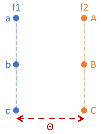
而兩個 \(\gamma\) 對應到兩種 搬運配對法
$$\begin{align*}
\gamma_1(a,A)=\gamma_1(b,B)=\gamma_1(c,C)=1/3 \\\\
\gamma_2(a,B)=\gamma_2(b,C)=\gamma_2(c,A)=1/3
\end{align*}$$
可以很容易知道它們的 marginal distributions 正好符合 f1 and f2 的機率分佈。
則這兩種搬運法造成的 EM distance 分別如下:
$$\begin{align*}
EM_{\gamma_1}=\gamma_1(a,A)*\Vert a-A \Vert + \gamma_1(b,B)*\Vert b-B \Vert + \gamma_1(c,C)*\Vert c-C \Vert \\\\
EM_{\gamma_2}=\gamma_2(a,B)*\Vert a-B \Vert + \gamma_2(b,C)*\Vert b-C \Vert + \gamma_2(c,A)*\Vert c-A \Vert
\end{align*}$$
明顯知道 $\theta=EM_{\gamma_1}<EM_{\gamma_2}$
而 EM distance 就是在算所有搬運法中,最小的那個,並將那最小的 cost 定義為此兩機率分佈的距離。
這個距離如果是兩條平行 1 維的直線 pdf (上面的例子是直線上只有三個離散資料點),會有如下的 cost:
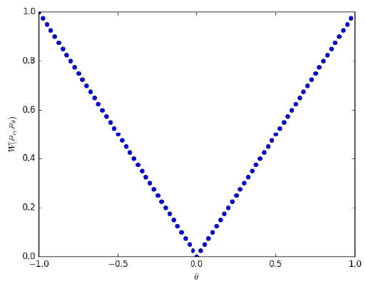
對比此圖和上一篇的 JSD 的結果,EM 能夠正確估算兩個沒有交集的機率分佈的距離,直接的結果就是 gradient 連續且可微 ! 使得 WGAN 訓練上穩定非常多。
一個關鍵的好性質: Wasserstein (Earth-Mover) distance 處處連續可微
原始 EM distance 的定義 (式(1)) 是 intractable
一個神奇的數學公式 (Kantorovich-Rubinstein duality) 將 EM distance 轉換如下:
$$\begin{align}
W(\mathbb{P}_r,\mathbb{P}_\theta)=\sup_{\Vert f \Vert _L \leq 1}{ E_{x \sim \mathbb{P}_r}[f(x)] - E_{x \sim \mathbb{P}_\theta}[f(x)] }
\end{align}$$
注意到 sup 是針對所有滿足 1-Lipschitz 的 functions f,如果改成滿足 K-Lipschitz 的 functions,則值會相差一個 scale K。
但是在實作上我們都使用一個 family of functions,例如使用所有二次式的 functions,或是 Mixture of Gaussians,等等。
而經過近幾年深度學習的發展後,我們可以相信,使用 DNN 當作 family of functions 是很洽當的選擇,因此假定我們的 NN 所有參數為 \(W\),則上式可以表達成:
$$\begin{align}
W(\mathbb{P}_r,\mathbb{P}_\theta)\approx\max_{w\in W}{ E_{x \sim \mathbb{P}_r}[f_w(x)] - E_{z \sim p(z)}[f_w(g_{\theta}(z))] }
\end{align}$$
這裡不再是等式,而是逼近,不過 Deep Learning 優異的 Regression 能力是可以很好地逼近的。
我們還是需要保證整個 EM distance 保持處處連續可微分,這樣可以確保我們做 gradient-based 最佳化可以順利,針對這點,WGAN 作者很強大地證明完了,得到結論如下:
針對生成器 \(g_\theta\)
任何 feed-forward NN 皆可針對鑑別器 \(f_w\)
當 \(W\) 是 compact set 時,該 family of functions \(\{f_w\}\) 滿足 K-Lipschitz for some K。
具體實現很容易,因為在 \(R^d\) space,compact set 等價於 closed and bounded,因此只需要針對所有的參數取 bounding box即可!
論文裡使用了 [-0.01,0.01] 這個範圍做 clipping。
與 GAN 第一個不同點為: 鑑別器參數取 clipping。
EM distance 為目標函式所造成的不同
我們將兩者的目標函式列出來做個比較
$$\begin{align}
GAN: E_{x \sim \mathbb{P}_r} [\log f_w(x)] + E_{z \sim p(z)}[\log (1-f_w(g_{\theta}(z)))] \\
WGAN: E_{x \sim \mathbb{P}_r}[f_w(x)] - E_{z \sim p(z)}[f_w(g_{\theta}(z))]
\end{align}$$
發現到 WGAN 不取 log,同時對生成器的目標函式也做了修改
與 GAN 第二個不同點為: WGAN 的目標函式不取 log,同時對生成器的目標函式也做了修改。
第三個不同點是作者實驗的發現
與 GAN 第三個不同點為: 使用 Momentum 類的演算法,如 Adam,會不穩定,因此使用 SGD or RMSProp。
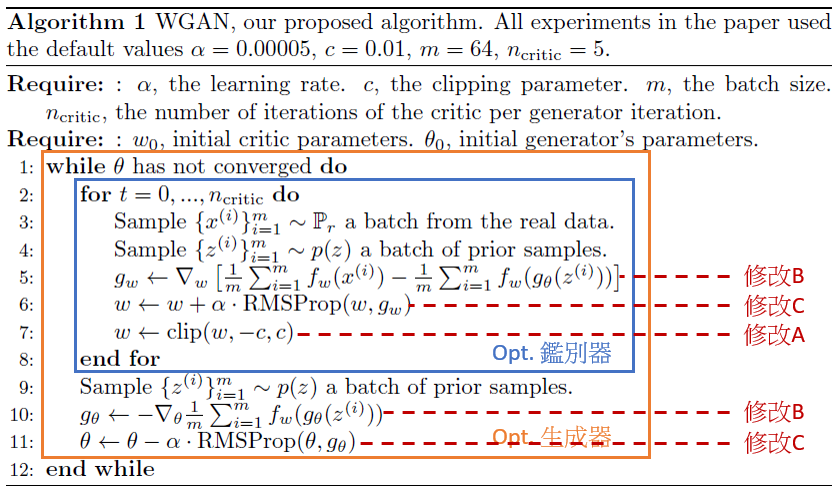
WGAN 演算法
總結一下與 GAN 的修改處
A. 鑑別器參數取 clipping。
B. WGAN 的目標函式不取 log,同時對生成器的目標函式也做了修改。
C. 使用 SGD or RMSProp。
WGAN 的優點
一: 目標函式與訓練品質高度相關
原始的 GAN 沒有這樣的評量指標,因此會在訓練中途用人眼去檢查訓練是否整個壞掉了。 WGAN 解決了這個麻煩。作者的範例如下,可以發現WGAN的目標函式 Loss 愈低,sampling出來的品質愈高。

二: 鑑別器可以直接訓練到最好
原始的 GAN 需要小心訓練,不能一下子把鑑別器訓練太強導致導函數壞掉
三: 不需要特別設計 NN 的架構
GNN 使用 MLP (Fully connected layers) 難以訓練,較成功的都是 CNN 架構,並搭配 batch normalization。而在 WGAN 演算法下, MLP架構可能穩定訓練 (雖然品質有下降)
四: 沒有 collapse mode (保持生成多樣性)
作者自己說在多次實驗的過程都沒有發現這種現象
My Questions
- 原先 GAN 會有 collapse mode 看到有人討論是因為 KL divergence 不對稱的關係導致對於 “生成器生出錯誤的 sample” 比 “生成器沒生出所有該對的sample” 逞罰要大很多,不過這邊自己還是有疑問,因為 JSD 已經是對稱的 KL 了,還會有逞罰不同導致 collapse mode 的問題嗎? 需要再多看一下 paper 了解。
- 如何控制 sample 出來的 output,譬如 mnist 要 sampling 出某個 class。前提是希望不能對 data 有任何標記過,不然就沒有 unsupervised 的條件了。 Conditional GAN? 有空再研究一下這個課題
Tensorflow 範例測試
主要參考此 github,用自己的寫法寫一次,並做些測試
用 MNIST dataset 做測試,原始 input 為 28x28,將它 padding 成 32x32,因此 input domain 為 32x32x1
生成器
幾個重點,第一個是生成器用的是conv2d_transpose(doc),這是由於原先的conv2d無法將 image 的 size 變大,頂多一樣。因此要用conv2d_transpose,以 第 15 行舉例。
argumentwc2的 shape 為[3, 3, 256, 512]分別表示[filter_h, filter_w, output_depth, input_depth]。argument[batch_size, 8, 8, 256]表示 output layer 的 shape。後面兩個 argument 就很明顯了,分別是 strides[batch_stride, h_stride, w_stride, channel_stride]和 padding。
第二個重點是最後一層out_sample = tf.nn.tanh(conv5),由於我們會將 data 先 normalize 到[-1,1],因此使用tanh讓 domain 一致。123456789101112131415161718192021222324252627282930313233z_dim = 128def generator_net(z):with tf.variable_scope('generator'):# Layer 1 - 128 to 4*4*512wd1 = tf.get_variable("wd1",[z_dim, 4*4*512])bd1 = tf.get_variable("bd1",[4*4*512])dense1 = tf.add(tf.matmul(z, wd1), bd1)dense1 = tf.nn.relu(dense1)# reshape to 4*4*512conv1 = tf.reshape(dense1, (batch_size, 4, 4, 512))# Layer 2 - 4*4*512 to 8*8*256wc2 = tf.get_variable("wc2",[3, 3, 256, 512])conv2 = tf.nn.conv2d_transpose(conv1, wc2, [batch_size, 8, 8, 256], [1,2,2,1], padding='SAME')conv2 = tf.nn.relu(conv2)# Layer 3 - 8*8*256 to 16*16*128wc3 = tf.get_variable("wc3",[3, 3, 128, 256])conv3 = tf.nn.conv2d_transpose(conv2, wc3, [batch_size, 16, 16, 128], [1,2,2,1], padding='SAME')conv3 = tf.nn.relu(conv3)# Layer 4 - 16*16*128 to 32*32*64wc4 = tf.get_variable("wc4",[3, 3, 64, 128])conv4 = tf.nn.conv2d_transpose(conv3, wc4, [batch_size, 32, 32, 64], [1,2,2,1], padding='SAME')conv4 = tf.nn.relu(conv4)# Layer 5 - 32*32*64 to 32*32*1wc5 = tf.get_variable("wc5",[3, 3, 1, 64])conv5 = tf.nn.conv2d_transpose(conv4, wc5, [batch_size, 32, 32, 1], [1,1,1,1], padding='SAME')out_sample = tf.nn.tanh(conv5)return out_sample鑑別器
這個就是最一般的 CNN,output 最後是一個沒有過 log 的 scaler 且也沒有經過 activation function。比較重要的是變數都是使用get_variable和scope.reuse_variables()(請參考 Sharing Variables)。
具體的原因是因為我們會對 real data 呼叫一次鑑別器,而對於 fake data 也會在呼叫一次。若沒有 share variables,就會導致產生兩組各自的 weights。tf.get_variable()跟tf.Variable()差別在於如果已經有名稱一樣的變數時 get_variable() 不會再產生另一個變數,而會 share,但是要真的 share 還必須多一個動作reuse_variables確保不是不小心 share 到的。12345678910111213141516171819202122232425262728293031323334353637# Construct CriticNetdef conv2d(x, W, b, strides=1):x = tf.nn.conv2d(x, W, strides=[1, strides, strides, 1], padding='SAME')x = tf.nn.bias_add(x, b)return tf.nn.relu(x)def critic_net(x, reuse=False):with tf.variable_scope('critic') as scope:size = 64if reuse:scope.reuse_variables()# Layer 1 - 32*32*1 to 16*16*sizewc1 = tf.get_variable("wc1",[3, 3, 1, size])bc1 = tf.get_variable("bc1",[size])conv1 = conv2d(x, wc1, bc1, strides=2)# Layer 2 - 16*16*size to 8*8*size*2wc2 = tf.get_variable("wc2",[3, 3, size, size*2])bc2 = tf.get_variable("bc2",[size*2])conv2 = conv2d(conv1, wc2, bc2, strides=2)# Layer 3 - 8*8*size*2 to 4*4*size*4wc3 = tf.get_variable("wc3",[3, 3, size*2, size*4])bc3 = tf.get_variable("bc3",[size*4])conv3 = conv2d(conv2, wc3, bc3, strides=2)# Layer 4 - 4*4*size*4 to 2*2*size*8wc4 = tf.get_variable("wc4",[3, 3, size*4, size*8])bc4 = tf.get_variable("bc4",[size*8])conv4 = conv2d(conv3, wc4, bc4, strides=2)# Fully connected layer - 2*2*size*8 to 1wd5 = tf.get_variable("wd5",[2*2*size*8, 1])bd5 = tf.get_variable("bd5",[1])fc5 = tf.reshape(conv4, [-1, wd5.get_shape().as_list()[0]])logit = tf.add(tf.matmul(fc5, wd5), bd5)return logitGraph
這裡有幾個重點,第一個是由於我們在最佳化過程中,會 fix 住一邊的參數,然後最佳化另一邊,接著反過來。此作法參考 link
第二個重點是使用tf.clip_by_value,可以看到我們對於所有透過tf.get_collection蒐集到的變數都增加一個 clip op。
第三個重點是使用tf.control_dependencies([opt_c])link,這個定義了 op 之間的關聯性,它會等到 argument 內執行完畢後,才會接著執行下去。
所以我們可以確保先做完RMSPropOptimizer才接著做clip_by_value。另外tf.tuplelink 會等所有的 input arguments 都做完才會真的 return 出去,以確保每個 tensors 都做完 clipping 了。1234567891011121314151617181920212223242526272829# build graphdef build_graph():z = tf.placeholder(tf.float32, shape=(batch_size, z_dim))fake_data = generator_net(z)real_data = tf.placeholder(tf.float32, shape=(batch_size, 32, 32, 1))# Define loss and optimizerreal_logit = critic_net(real_data)fake_logit = critic_net(fake_data, reuse=True)c_loss = tf.reduce_mean(fake_logit - real_logit)g_loss = tf.reduce_mean(-fake_logit)# get the trainable variables listtheta_g = tf.get_collection(tf.GraphKeys.TRAINABLE_VARIABLES, scope='generator')theta_c = tf.get_collection(tf.GraphKeys.TRAINABLE_VARIABLES, scope='critic')# freezing or only update designated variablesopt_g = tf.train.RMSPropOptimizer(learning_rate=lr_generator).minimize(g_loss, var_list=theta_g)opt_c = tf.train.RMSPropOptimizer(learning_rate=lr_critic).minimize(c_loss, var_list=theta_c)# then pass those trainable variables to clip functionclipped_var_c = [tf.assign(var, tf.clip_by_value(var, clip_lower, clip_upper)) for var in theta_c]# wait until RMSPropOptimizer is donewith tf.control_dependencies([opt_c]):# fetch the clipped variables and output as opopt_c = tf.tuple(clipped_var_c)return opt_g, opt_c, z, real_dataWGAN Algorithm Flow
照 paper 上的演算法 flow123456789101112131415161718192021222324252627282930def wgan_train():dataset = input_data.read_data_sets(".", one_hot=True)opt_g, opt_c, z, real_data = build_graph()saver = tf.train.Saver()config = tf.ConfigProto(allow_soft_placement=True, log_device_placement=True)config.gpu_options.allow_growth = Trueconfig.gpu_options.per_process_gpu_memory_fraction = 0.8def next_feed_dict():train_img = dataset.train.next_batch(batch_size)[0]train_img = 2*train_img-1train_img = np.reshape(train_img, (-1, 28, 28))npad = ((0, 0), (2, 2), (2, 2))train_img = np.pad(train_img, pad_width=npad,mode='constant', constant_values=-1)train_img = np.expand_dims(train_img, -1)batch_z = np.random.normal(0, 1, [batch_size, z_dim]).astype(np.float32)feed_dict = {real_data: train_img, z: batch_z}return feed_dictwith tf.Session(config=config) as sess:sess.run(tf.global_variables_initializer())summary_writer = tf.summary.FileWriter(log_dir, sess.graph)for i in range(max_iter_step):print("itr = ",i)for j in range(c_iter):feed_dict = next_feed_dict()sess.run(opt_c, feed_dict=feed_dict)feed_dict = next_feed_dict()sess.run(opt_g, feed_dict=feed_dict)if i % 1000 == 999:saver.save(sess, os.path.join(ckpt_dir, "model.ckpt"), global_step=i)一點小結論
5.1. 上述架構沒有用 batch normalization,有用的話效果會好很多,生成器和鑑別器都可用。
5.2. 鑑別器換成其他 CNN 架構也可以。
5.3. MLP 架構也可以。
整體來說,對於熟悉 tensorflow 的人來說不難實作 (剛好我不是很熟),尤其 WGAN 從根本上做的改進,讓整個 training 很容易!
讓我們期待接下來的發展吧~
Reference
- GAN
- Wasserstein GAN,作者的 github
- 令人拍案叫绝的Wasserstein GAN
- A Tensorflow Implementation of WGAN: 使用
tf.contrib.layers,一個 higher level 的 API,比我現在的實作可以簡潔很多。 - A GENTLE GUIDE TO USING BATCH NORMALIZATION IN TENSORFLOW: Batch Normalization, MLP, and CNN examples using tf.contrib.layers