這是一篇論文Learning Sparse Neural Networks through L0 Regularization 的詳細筆記, 同時自己實作做實驗 [My Github]
主要以詳解每個部分並自己能回憶起為目的, 所以或許不是很好閱讀
Introduction
NN model 參數 $\theta$, 我們希望非$0$的個數愈少愈好, i.e. $|\theta|_0$ 愈小愈好, 所以會加如下的 regularization term:
$$\mathcal{L}_C^0(\theta)=\|\theta\|_0=\sum_{j=1}^{|\theta|}\mathbb{I}[\theta_j\neq0]$$ 所以 Loss 為:
但實務上我們怎麼實現 $\theta$ 非 $0$ 呢?
一種方式為使用一個 mask random variable $Z=\{Z_1,...,Z_{|\theta|}\}$ (~Bernoulli distribution, 參數 $q=\{q_1,...,q_{|\theta|}\}$), 因此 Loss 改寫如下: (注意到 $\mathcal{L}_C^0$ 可以有 closed form 並且與 $\theta$ 無關了)
現在最大的麻煩是 entropy loss $\mathcal{L}_E$, 原因是 Bernoulli 採樣沒辦法對 $q$ 微分, 因為 $\nabla_q\mathcal{L}_E(\theta,q)$ 在計算期望值時, 採樣的機率分佈也跟 $q$ 有關
參考 Gumbel-Max Trick 開頭的介紹說明
好消息是, 可以藉由 reparameterization (Gumbel Softmax) 方法使得採樣從一個與 $q$ 無關的 r.v. 採樣 (所以可以微分了), 因此也就能在 NN 訓練使用 backpropagation.
以下依序說明: (參考這篇 [L0 norm稀疏性: hard concrete门变量] 整理的順序, 但補足一些內容以及參考論文的東西)
Gumbel max trick $\Rightarrow$ Gumbel softmax trick (so called concrete distribution)
$\Rightarrow$ Binary Concrete distribution $\Rightarrow$ Hard (Binary) Concrete distribution $\Rightarrow$ L0 regularization
最後補上對 GoogleNet 架構加上 $L0$ regularization 在 CIFAR10 上的模型壓縮實驗
文長…
Gumbel Distribution
$G\sim\text{Gumbel}(\mu,\beta)$, 其 CDF $F(x)$ 為
$$F(x):=P(G\leq x)=e^{-e^{-(x-\mu)/\beta}}$$
當 $\mu=0,\beta=1$ 時為 standard Gumbel r.v., 所以 CDF 為 $\exp{(-\exp{(-x)}})$ [wiki]

CDF 是一個 monotonely increasing function, 存在 inverse function:
$$\begin{align} F^{-1}(F(x))=x \Rightarrow F^{-1}\left(e^{-e^{-(x-\mu)/\beta}}\right)=x \\ \Longrightarrow F^{-1}(p)= \mu-\beta\ln(-\ln(p)) \end{align}$$CDF 的 inverse function 又稱 quantile function (Help me understand the quantile (inverse CDF) function)
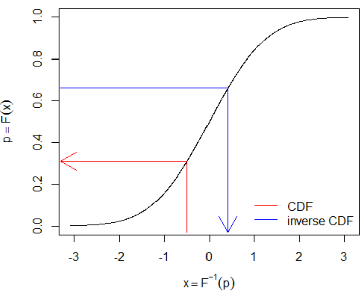
所以如果 $F^{-1}(U)$ where $U\sim\text{Uniform}(0,1)$, 等於照機率分佈取 Gumbel random variable.
- Inverse transform sampling [wiki]
假設有一個 strictly monotone transfromation (所以存在 inverse) $T:[0,1]\rightarrow\mathbb{R}$, 使得 $T(U)=_dX$, 其中 $U\sim\text{Uniform}(0,1)$. 那我們就可以使用 $T$ 來做 $X$ 的採樣
令 $X$ 的 CDF 為 $F_X(x)$, 則:
$$F_X(x)=Pr(X\leq x)=Pr(T(U)\leq x) \\ =Pr(U\leq T^{-1}(x))=T^{-1}(x)$$ 則我們發現 $T$ 是 $F_X^{-1}$. 因此 $F_X^{-1}(U)$ 就可以用來採樣 $X$.
Let $U\sim\text{Uniform}(0,1)$, then $F^{-1}(U)=\mu-\beta\ln(-\ln(U))\sim\text{Gumbel}(\mu,\beta)$.
另外, 兩個 Gumbel r.v.s 的 difference 服從 Logistic distribution.
If $X\sim\text{Gumbel}(\mu_X,\beta)$ and $Y\sim\text{Gumbel}(\mu_Y,\beta)$ are independent, then, $X-Y\sim\text{Logistic}(\mu_X-\mu_Y, \beta)$
Logistic random variable 其 CDF 是 sigmoid function.
Categorical Distribution and Gumbel Max Trick
$X\sim\text{Categorical}(\alpha_1,\alpha_2,...,\alpha_n)$ 表示取到第 $i$ 類的機率是 $\alpha_i$.
並且有如下的 reparameterization 方式:
$$X'\sim\arg\max\left(G_1+\ln\alpha_1,...,G_n+\ln\alpha_n\right)$$ 其中 $(G_1,...,G_n)$ 為 $n$ 個獨立的 Gumbel r.v.s.
則 $X=_dX’$.
Concrete Random Variable
簡單講, 將 Gumbel max trick 中的 $\arg\max$ 改成 softmax (with temperature $\tau$)
$$X\sim\text{Concrete}((\alpha_1,\alpha_2,..,\alpha_n),\tau)$$ 其中 $\tau\in(0,\infty)$ and $\alpha_k\in(0, \infty)$.
則 $X$ 的取法為:
1. Sample $n$ 個獨立的 Gumbel r.v.s: $(g_1,...,g_n)\sim(G_1,...,G_n)$, 視為 Gumbel noises
2. 將 logits, $\ln\alpha_k$, 加上這 $n$ 個 Gumbel noises 並做 softmax (with temperature $\tau$) 成為 distribution: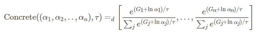
更多請參考 The Concrete Distribution: A Continuous Relaxation of Discrete Random Variables
簡而言之, Concrete distirbution 是將 discrete 的 categorical r.v. relax 成 continuous 版本, 意即取出來的 random variable 不再是 simplex 的 one-hot 形式, 而是連續的數值, 論文裡的圖示很清楚 (圖中的 $\lambda$ 為 temperature $\tau$)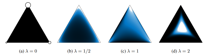
當 $\tau\rightarrow 0$, 則 concrete distribution 變成 categorical distribution.
Binary Concrete Distribution
Concrete distribution 只剩下 binary 的話, 可以做化簡剩兩個參數 $(\alpha,\tau)$.
$$X=(X_1,X_2)\sim\text{Concrete}((\alpha_1,\alpha_2),\tau), \\
(X_1,X_2)\sim\left[\frac{e^{(G_1+\ln\alpha_1)/\tau}}{e^{(G_1+\ln\alpha_1)/\tau}+e^{(G_2+\ln\alpha_2)/\tau}},\frac{e^{(G_2+\ln\alpha_2)/\tau}}{e^{(G_1+\ln\alpha_1)/\tau}+e^{(G_2+\ln\alpha_2)/\tau}}\right] \\
\Longrightarrow X_1\sim\frac{e^{(G_1+\ln\alpha_1)/\tau}}{e^{(G_1+\ln\alpha_1)/\tau}+e^{(G_2+\ln\alpha_2)/\tau}} = \frac{1}{1+e^{(G_2-G_1+\ln\alpha_2-\ln\alpha_1)/\tau}} \\
=\sigma\left(\frac{G_1-G_2+\ln\alpha_1-\ln\alpha_2}{\tau}\right) = \sigma\left(\frac{L+\ln\alpha_1-\ln\alpha_2}{\tau}\right)\\
=\sigma\left(\frac{L+\ln(\alpha_1/\alpha_2)-{\color{orange}0}}{\tau}\right)=\sigma\left(\frac{L+\ln(\alpha_1/\alpha_2)-{\color{orange}\ln1}}{\tau}\right)
$$ 其中 $\sigma(x)=1/(1+e^{-x})$ 為 sigmoid function, 且已知兩個 Gumbel r.v.s 相減, $(G_1-G_2)=L\sim \text{Logistic}$, 是 Logistic, 而 $L=\ln U-\ln(1-U)$, where $U\sim\text{Uniform}(0,1)$.
想成 $\alpha_1'=\alpha_1/\alpha_2$, 且 $\alpha_2'=1$, 則 $X=(X_1,1-X_1)\sim\text{Concrete}((\alpha_1',\alpha_2'),\tau)$, 代入 $\alpha_2'=1$ 後把下標 $1$ 去掉得到 Binary Concrete random variable:
$$
\begin{align}
(X,1-X)\sim\text{Concrete}((\alpha,1),\tau)\\
\Longrightarrow
{\color{orange}{
X\sim\text{BinConcrete}(\alpha,\tau):=\sigma\left(\frac{L+\ln\alpha}{\tau}\right)
=\sigma\left(\frac{\ln U-\ln(1-U)+\ln\alpha}{\tau}\right)}
}
\end{align}
$$
圖改自 The Concrete Distribution: A Continuous Relaxation of Discrete Random Variables
可以觀察到 $\tau$ 愈接近 $0$, 則 $X$ 的值愈有可能是 $0$ or $1$ 的 binary case.
Binary Concrete 的 CDF 為 ${\color{orange}{P(X<x)=\sigma(\tau(\ln x-\ln(1-x))-\ln\alpha)}}$ 推導如下: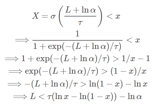
已知 $L\sim \text{Logistic}$, 所以 $P(L<\tau(\ln x-\ln(1-x))-\ln\alpha)=\sigma(\tau(\ln x-\ln(1-x))-\ln\alpha)$
官方 implementation [codes]
Hard (Binary) Concrete Distribution
主要就是將 Binary concrete r.v. 拉伸平移, 並 clip 在 $(0,1)$ 區間
Hard binary concrete r.v. 取法為:
1. $X\sim\text{BinConcrete}(\alpha,\tau)=\sigma\left((\ln U-\ln(1-U)+\ln\alpha)/\tau\right)$.
2. Stretch: $\bar{X}=X(b-a)+a$, 將 $X$ 拉伸平移.
3. Hard-sigmoid to produce Gating r.v.: $Z=\min(1,\max(0,\bar{X}))$.
其中 $a<0<1<b$.
當 $0<X<-a/(b-a)$, 則 $Z=0$,
當 $(1-a)/(b-a)<X<1$, 則 $Z=1$,
否則 $(1-a)/(b-a)<X<-a/(b-a)$, $Z=\bar{X}$.
Stretch + hard-sigmoid functions 是為了把 Binary Concrete random variable 真的是 $0$ or $1$ 的機會再變更大
請參考 “Binary Concrete Distribution” 段落裡的圖就能想像
所以 $P(Z=0)=P(X<-a/(b-a))$.
我們由 Binary Concrete 的 CDF 為 $P(X<x)=\sigma(\tau(\ln x-\ln(1-x))-\ln\alpha)$ 可以得知:
$$
{\color{orange}{P(Z\neq0)}}=1-P\left(X<\frac{-a}{b-a}\right) \\
=1-\sigma\left(\tau\left(\ln \frac{-a}{b-a}-\ln\left(1-\frac{-a}{b-a}\right)\right)-\ln\alpha\right) \\
=1-\sigma\left(-\ln\alpha+\tau\ln\frac{-a}{b}\right)
{\color{orange}{=\sigma\left(\ln\alpha-\tau\ln\frac{-a}{b}\right)}}
$$ 所以最後 Gating random variable $Z\neq0$ 的機率, $P(Z\neq0)$, 我們可以得到 closed form.
$\mathcal{L}_0$ Regularization
$P(Z\neq0)$ 其實這就是 $L_0$ regularization term 了!
$$
\mathcal{L}_C^0(\phi)=\sum_j P(Z_j\neq0|\phi_j)=\sum_j \sigma\left(\ln\alpha_j-\tau_j\ln\frac{-a}{b}\right)
$$ 其中 $\phi_j=\{\alpha_j,\tau_j\}$ 表示 Binary Concrete r.v. 的參數
實務上 $\ln\alpha_j$ 是 learnable 的參數, 而 $\tau_j$ 一般直接給定
而原本的 loss 就是 weights $\theta$ 乘上 gating variable $Z$:
注意到 $\text{BinConcrete}$ 可以藉由 reparameterization trick (變成 sample 這個 operation 跟參數無關, i.e. 利用 standard Uniform or Logistic r.v.s 取 samples) 來做 backpropagation.
Total loss 就是
$$
\mathcal{L}(\theta,\phi)=\mathcal{L}_E(\theta,\phi)+\lambda\mathcal{L}_C^0(\phi)
$$
論文考慮了如果加入 L2-norm 的 regularization 怎麼改動.
原本的 $\mathcal{L}_2$ regularization 只是參數的 square: $\sum_j \theta_j^2$, 但為了跟 $\mathcal{L}_0$ 有個比較好的結合, 改成如下: (細節請參考論文)
$$
\mathcal{L}_C^2(\theta,\phi)=\sum_j \theta_j^2 P(Z_j\neq0|\phi_j)
$$
所以結合後的 regularization term 如下:
$$
\mathcal{L}_C(\theta,\phi)=\lambda_2\cdot 0.5\cdot\mathcal{L}_C^2(\theta,\phi)+\lambda_0\cdot\mathcal{L}_C^0(\phi) \\
= \sum_j \left( \lambda_2\cdot0.5\cdot\theta_j^2 + \lambda_0
\right)P(Z_j\neq0|\phi_j)
$$
因此 Total loss 就是
$$
\mathcal{L}(\theta,\phi)=\mathcal{L}_E(\theta,\phi)+\lambda\mathcal{L}_C(\theta,\phi)
$$
Experimental Codes and Results
Network Structure
使用 GoogleNet 在 CIFAR10 上做實驗 [Github repo]
具體怎麼做 L0 purning 呢? 以 convolution 舉例, 我們對 output channel 做 masking, 因此每個 channel 會對應一個 hard binary concrete r.v. $Z_i$, 由於 hard binary concrete r.v. 傾向 sample 出 exactly $0$ or $1$ (中間數值也有可能, 只是很低機率), 因此造成 output dimension 會直接下降, 所以給下一層的 layer 的 channel 數量就減少, 圖示如下: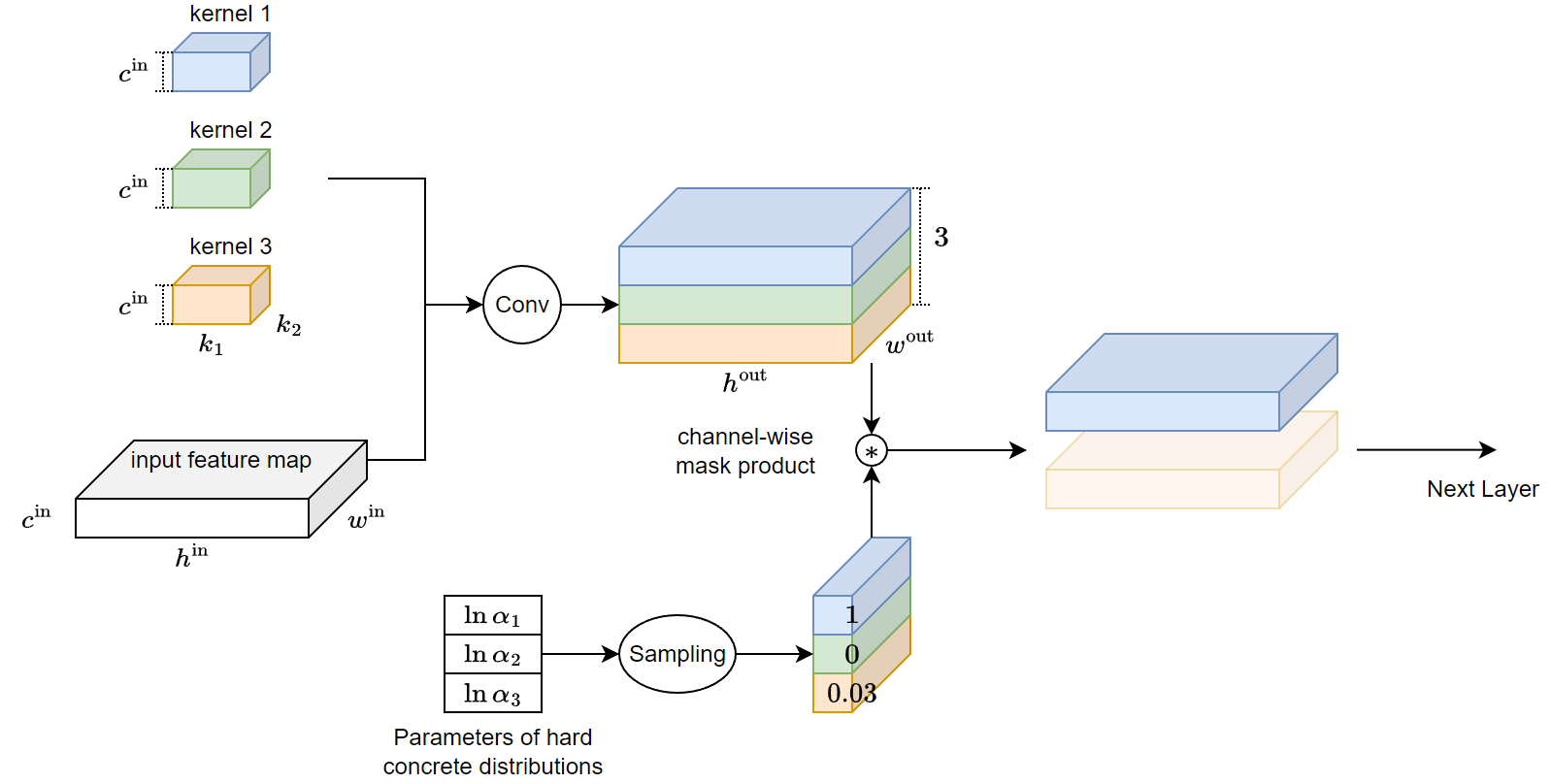
有關 hard concrete r.v. 的 module 參考 class L0Gate(nn.Module) [link]
因此 Inception block 會多了一些 L0Gate layers: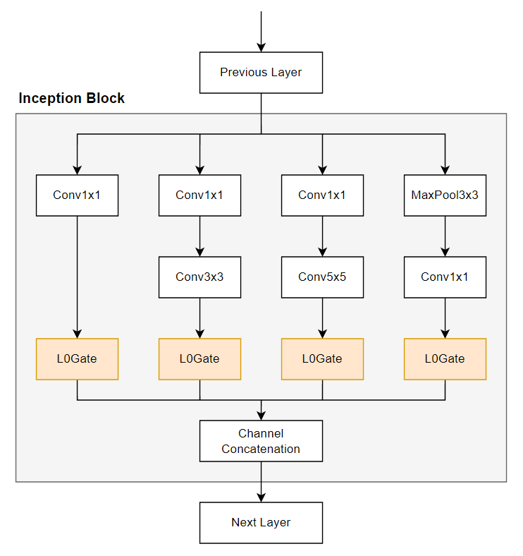
所以 inception layer 的 forward() 大概就是長這樣: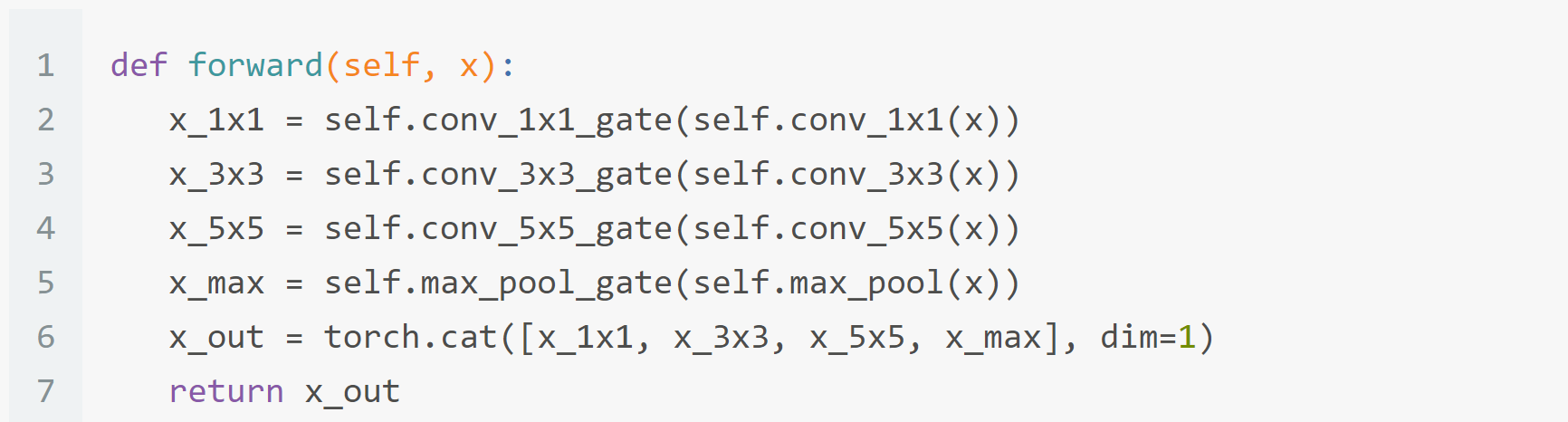
再來就是用這些包含 L0Gate 的 inception blocks 去建立整個 GoogleNet 的 NN 了.
Results
Recap 一下 Loss:
$$
\mathcal{L}(\theta,\phi)=\mathcal{L}_E(\theta,\phi)+\lambda\mathcal{L}_C^0(\phi)
$$ 其中 $\phi_j=\{\alpha_j,\tau_j\}$ 表示 Binary Concrete r.v. 的參數, 一般來說只有 $\ln\alpha_j$ 是 learnable, 而 $\lambda$ 表示 L0 regularization 的比重
我們將 L0Gate 的參數, i.e. $\ln\alpha_j$, 與 NN 的參數 $\theta$ 一起從頭訓練起
對比沒有 L0 regularization 的就是原始的 GoogleNet
| GoogleNet | Validation Accuracy | Test Accuracy | Sparsity |
|---|---|---|---|
| NO L0 | 90.12% | 89.57% | 1.0 |
| with L0, lambda=0.25 | 88.66% | 87.87% | 0.94 |
| with L0, lambda=0.5 | 86.9% | 86.56% | 0.78 |
| with L0, lambda=1.0 | 83.2% | 82.79% | 0.45 |
其中 sparsity 的計算為所有因為 gate 為 $0$ 而造成參數無效的比例
可以觀察到隨著 $\lambda$ 愈大, 會 pruning 更多 ($\mathcal{L}_C^0$ 的收斂值會更低), 但也造成 accuracy 的下降
對比下面的圖也可以看到 $\lambda$ 對 $\mathcal{L}_C^0$ 的收斂值的影響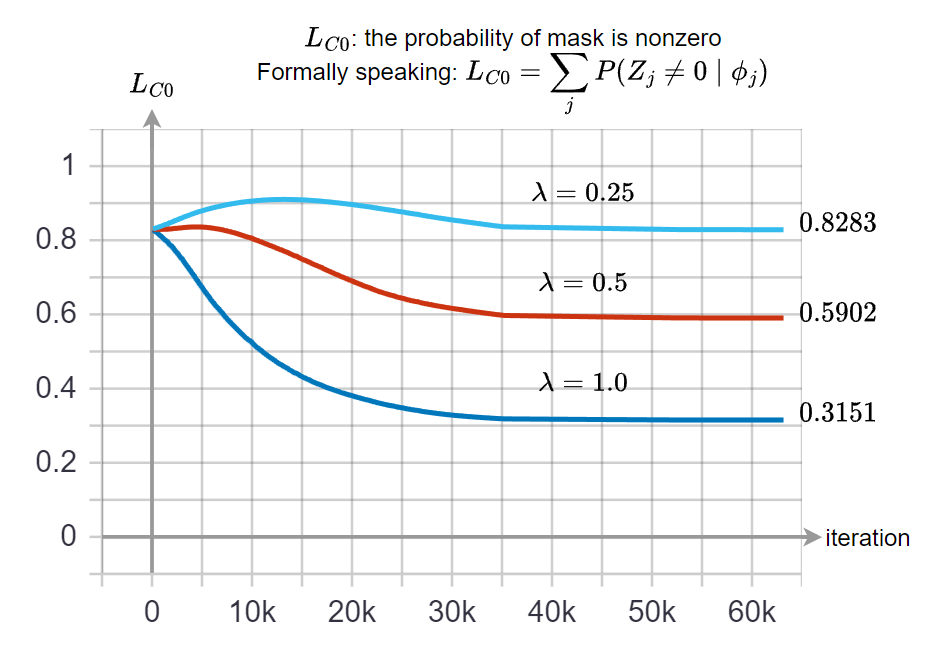 實務上乘 gate $0$ 等於事先將 weight 變成 $0$, 而因為我們使用 structure pruning, 所以可以將 convolution kernel 變小.
後來我發現比起將 $\ln\alpha_j$, 與 NN 的參數 $\theta$ 一起從頭訓練起
NN $\theta$ init 使用之前 pre-train 好的 model (沒有 L0), 然後再加入 L0 regularization, 此時將 $\ln\alpha$ 初始成比較大的值 (接近 $1$, i.e. 讓 gate 打開), 這樣在同樣 sparsity 效果下, accuracy 會比較高
References
- L0 norm稀疏性: hard concrete门变量
- The Concrete Distribution: A Continuous Relaxation of Discrete Random Variables
- L0 Regularization Practice [My Github]
- In paperswithcode: [link]
- Pruning Filters & Channels in Neural Network Distiller