先引用這篇論文的論點 Train Large, Then Compress: Rethinking Model Size for Efficient Training and Inference of Transformers [pdf]
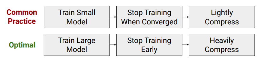
同樣的小 model size, 從頭訓練還不如先用大的 model size 做出好效果, 再壓縮到需要的大小
所以 pruning 不僅能壓小 model size, 同樣對 performance 可能也是個好策略
Introduction
使用單純的 absolutely magnitude pruning 對於在 SSL model 不好. 因為原來的 weight 是對 SSL 的 loss 計算的, 並不能保證後來的 fine tune (down stream task loss) 有一樣的重要性關聯.
例如傳統上的 magnitude pruning 作法, 如這一篇 2015 NIPS 文章 [Learning both Weights and Connections for Efficient Neural Networks] (cited 5xxx) 作法很簡單:
先對 model train 到收斂, 然後 prune, 接著繼續訓練 (prune 的 weight 就 fix 為 $0$), 然侯再多 prune … iterative 下去到需要的 prune 數量
但作者認為, 只靠 magnitude 大小判斷效果不好, 因為在 fine tune 過程中, 如果某一個 weight 雖然 magnitude 很大, 但 gradient update 後傾向把 magnitude 變小, 就表示它重要性應該降低才對, 這是本篇的精華思想
因此我們先定義重要性就是代表 weight 的 magnitude 會變大還是變小, 變大就是重要性大, 反之
因此作者對每一個參數都引入一個 score, 命為 $S$, 希望能代表 weight 的重要性. 而在 fine-tune 的過程, 除了對 weight $W$ update 之外, score $S$ 也會 update
如果 score $S$ 正好能反映 weight 的 gradient 傾向, 即 $S$ 愈大剛好表示該對應的 weight 在 fine-tune 過程會傾向讓 magnitude 變大, 反之亦然, 那這樣的 $S$ 正好就是我們要找的.
要這麼做的話, 我們還需要回答兩個問題:
- 怎麼引入 score $S$?
- Score $S$ 正好能代表重要性? 換句話說能反映 weight 在 fine tune 過程的 magnitude 傾向嗎?
怎麼引入 score $S$?
首先, 看一下 $W$ and $S$ 的 gradients
Forward:
$$
a=(W\odot M)x
$$
$W$是 weight matrix, 而 $M$是 mask matrix 每一個 element $\in\{0,1\}$, $M$ 通常是從一個 score matrix $S$ 搭配上 masking function e.g. $\text{Top}_v$ 而來:
$$M_{ij}=\text{Top}_v(S)_{ij}=\left\{
\begin{array}{ll}
1, & S_{ij}\quad\text{in top }v\% \\
0, & \text{o.w.}
\end{array}
\right.$$ 而 magnitude based pruning 定義 $S_{ij}=|W_{ij}|$
算 $W$ 的 gradients:
$$\begin{align}
\frac{\partial L}{\partial W_{ij}}=\frac{\partial L}{\partial a_i}M_{ij}x_{j}
\end{align}$$
而算 $S$ 的 gradients 時發現因為 $\text{Top}_v$ 無法微分
所以用 straight-through estimator (STE), i.e. 假裝沒有 $\text{Top}_v$ 這個 function.
修改為可微分的 forward:
改成讓 forward 假裝沒有過 $\text{Top}_v$ (因為 $\text{Top}_v$ 無法微分):
$$
a=(W\odot {\color{orange}S})x
$$
所以 $S$ 的 gradients:
$$\begin{align}
\frac{\partial L}{\partial S_{ij}} = \frac{\partial L}{\partial a_i}\frac{\partial a_i}{\partial S_{ij}}=\frac{\partial L}{\partial a_i}W_{ij}x_j
\end{align}$$
所以 $S$ 仍然會被 update, 就算對應的 weight 已經在 forward 被 mask 了
這種作法稱 Straigth Through Estimator (STE)
Appendix A.1 證明 training loss 會收斂 (原論文有幾個推導當下沒看懂, 後來自己補足了一些推導, 見本文最後面段落)
Score $S$ 能代表重要性?
先回顧一個觀念
$$\frac{\partial \mathcal{L}}{\partial W_{ij}}>0$$ 表示 loss function $\mathcal{L}$ 與 $W_{ij}$ 方向一致, 換句話說
$$\frac{\partial \mathcal{L}}{\partial W_{ij}}<0$$ 則表示方向相反
我們現在觀察 $S$ 和 $W$ 在 update 時候之間的關係, 由 (1) and (2) 的關係可以寫成如下:
$$\begin{align} \frac{\partial L}{\partial S_{ij}} = \frac{\partial L}{\partial W_{ij}}W_{ij} / M_{ij} \end{align}$$
首先我們注意到如果 $\partial L / \partial S_{ij} < 0$, 表示 $L$ 和 $S_{ij}$ 方向相反, 因為我們希望 $L\downarrow$, 所以此時 $S_{ij}\uparrow$.
要讓 $\partial L / \partial S_{ij} < 0$ 根據 (3) 只會有兩種情形 (我們不管 $M_{ij}$, 因為它 $\geq0$):
Case 1: $\partial L / \partial W_{ij} < 0$ and $W_{ij}>0$. Weight 是正的, 且它的行為跟 $L$ 方向相反. 所以更新後 weight 會變得更大 (away from zero)
Case 2: $\partial L / \partial W_{ij} > 0$ and $W_{ij}<0$. Weight 是負的, 且它的行為跟 $L$ 方向相同. 所以更新後 weight 會變得更小 (close to zero)
上述兩種 weight 都會離 $0$ 愈來愈遠 (magnitude 會變更大).
結論就是 update 過程如果 $S_{ij}\uparrow$ 表示 $W_{ij}$ 遠離 $0$.
同樣的推理, 如果 $\partial L / \partial S_{ij} > 0$, 表示 $S_{ij}\downarrow$ 的情形發生在 $W_{ij}$ 更靠近 $0$ 了.
所以我們得到一個結論:
因為 $S$ 升高對應到 $|W|$ 變大; $S$ 降低對應到 $|W|$ 變小. 所以合理認為 $S$ 代表的是重要性
有意思的是, 上述結論似乎跟 masking function 是否用 $\text{Top}_v$ 無關
意思是如果 masking function 用 $\text{Bottom}_v$ (選最小的那 $v\%$) 也會有 “$S$ 升高對應到 $W$ 變大; $S$ 降低對應到 $W$ 變小, 因此 $S$ 是重要性” 這個結論
但怎麼感覺哪裡怪怪的
不過其實邏輯上不衝突, 我這邊的理解是這樣的:
Score $S$ 代表重要性是沒問題的, 只是這個重要性現在只針對 $\text{Bottom}_v$ 的那些 weights 去看
同時, Appendix A.1 證明 loss 能收斂也是基於 $\text{Top}_v$ 能得到保證, 因此用 $\text{Bottom}_v$ 搞不好收斂不起來
$S$ 的更新過程可以視為 movement (重要性) 的累積 (只要初始給 $0$ ??)
Results
在 low sparsity (more than 70% of remaining weights), magnitude pruning 比 movement pruning 好
在 high sparsity (less than 15% of remaining weights), 則 movement pruning 好得很明顯

總體來說在 high sparsity case, Soft movement pruning (SMvP) > Movement Pruning (MvP) > L0 regularization > Magnitude Pruning (MaP)
作者強調了一下 MvP or SMvP 比 L0 簡單又更好
最後作者在 pruning 過程中加了 distillation loss, 顯示 distillation 對所有 pruning methods 都有幫助.
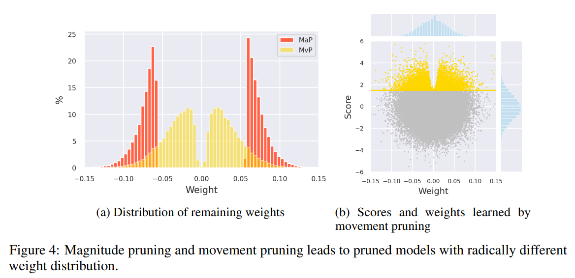
Fig 4(a) 不意外
Fig 4(b) 比較有意思, score 大的那些 weight 都不會 $0$ 靠近 (v-shape)
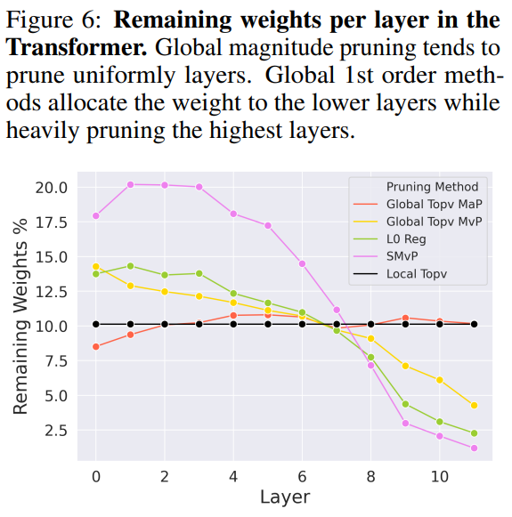
作者實驗了 global/local NN 的 pruning, 之前是說 global 讓 NN 自己決定每個 layers 要 prune 多少比例, 所以通常比較好 (尤其在 high sparsity)
但作者在自己的實驗, 發現兩者在效果上沒太大差異
最後分析一下每個 layer 的 sparsity, 發現在愈後面的 layer prune 愈多
Codes
HuggingFace 有實現這段 codes:
|
|
注意到繼承 autograd.Function 就要 implement forward and backward 方法, 讓它可以微分
我們可以看到 backward 什麼事都沒做, 這是因為 STE (Straight-Through Estimator) 的關係
所以在 forward 的時候 inputs tensor 就給 score matrix $S$, 這樣可以求出對應的 mask $M$, 同時這個 TopK 又可以微分
Appendix A.1 Guarantees on the decrease of the training loss
補充推導, 先回顧一下
Forward:
$$
a=(W\odot M)x
$$
針對 Backward relaxing 的 forward:
$$
a=(W\odot S)x
$$
其中 $M=\text{Top}_k(S)$, score matrix 經過選擇變成 mask matrix. 不失一般性, 我們定義 score 都為正, $S_{ij}>0$.
算 $W$ 的 gradients:
$$\frac{\partial L}{\partial W_{ij}}=\frac{\partial L}{\partial a_i}M_{ij}x_{j} \\
\frac{\partial L}{\partial W_{kl}}=\frac{\partial L}{\partial a_k}M_{kl}x_{l}$$
算 $S$ 的 gradients, 不過由於 $\text{Top}_k$ 無法算微分, 所以只好用 Backward relaxing 的替代方式
$$\frac{\partial L}{\partial S_{ij}} = \frac{\partial L}{\partial a_i}\frac{\partial a_i}{\partial S_{ij}}=\frac{\partial L}{\partial a_i}W_{ij}x_j \\ \frac{\partial L}{\partial S_{kl}} = \frac{\partial L}{\partial a_k}\frac{\partial a_k}{\partial S_{kl}}=\frac{\partial L}{\partial a_k}W_{kl}x_l$$ 要證明, movement pruning 算法造成的 $\text{Top}_k$ 變化, 仍會使得 loss 愈來愈低.先將問題簡化為 $\text{Top}_1$, 在 iteration $t$ 最高分的是 index $(i,j)$, i.e. $\forall u,v,S_{uv}^{(t)}\leq S_{ij}^{(t)}$. 然後 update 一次後, 變成 index $(k,l)$ 是最大.
$$\left\{ \begin{array}{ll} \text{At } t, & \forall1\leq u,v\leq n,\quad S_{uv}^{(t)}\leq S_{ij}^{(t)} \\ \text{At } t+1, & \forall1\leq u,v\leq n,\quad S_{uv}^{(t+1)}\leq S_{kl}^{(t+1)} \end{array} \right.$$
所以有 $S_{kl}^{(t+1)}-S_{kl}^{(t)} \geq S_{ij}^{(t+1)}-S_{ij}^{(t)}$.
我們從定義出發:
$$\frac{\partial L}{\partial S_{ij}^{(t)}}=\lim_{|\Delta|\rightarrow0}\frac{L\left(S^{(t+1)}\right) - L\left(S^{(t)}\right)}{S_{ij}^{(t+1)}-S_{ij}^{(t)}},\quad\text{where }\Delta=S_{ij}^{(t+1)}-S_{ij}^{(t)}$$
因此我們觀察兩次的 losses 差異:
$$L(a_i^{(t+1)},a_k^{(t+1)})-L(a_i^{(t)},a_k^{(t)}) \\ \\ \approx \frac{\partial L}{\partial a_k}(a_k^{(t+1)}-a_k^{(t)}) + \frac{\partial L}{\partial a_i}(a_i^{(t+1)}-a_i^{(t)}) \\ \\ =\frac{\partial L}{\partial a_k}W_{kl}^{(t+1)}x_l - \frac{\partial L}{\partial a_i}W_{ij}^{(t)}x_j \\ \\ = \frac{\partial L}{\partial a_k}W_{kl}^{(t+1)}x_l + (-\frac{\partial L}{\partial a_k}W_{kl}^{(t)}x_l + \frac{\partial L}{\partial a_k}W_{kl}^{(t)}x_l) - \frac{\partial L}{\partial a_i}W_{ij}^{(t)}x_j \\ \\ = \frac{\partial L}{\partial a_k}(W_{kl}^{(t+1)}x_l-W_{kl}^{(t)}x_l) + (\frac{\partial L}{\partial a_k}W_{kl}^{(t)}x_l - \frac{\partial L}{\partial a_i}W_{ij}^{(t)}x_j) \\ \\ = \underbrace{\frac{\partial L}{\partial a_k}x_l(-\alpha_W\frac{\partial L}{\partial a_k}x_lm(S^{(t)})_{kl})}_{\text{term1}=0} + \underbrace{(\frac{\partial L}{\partial a_k}W_{kl}^{(t)}x_l - \frac{\partial L}{\partial a_i}W_{ij}^{(t)}x_j)}_{\text{term2}<0}$$
第二行的 $\approx$ 使用泰勒展開式
二維的泰勒展開式
$$f(t_n+\Delta t,x_n+\Delta x)=f(t_n,x_n)+\left[\begin{array}{cc}f_t(t_n,x_n) & f_x(t_n,x_n)\end{array}\right]\left[\begin{array}{c}\Delta t \\ \Delta x\end{array}\right] + O\left( \left\| \left[\begin{array}{c}\Delta t \\ \Delta x\end{array}\right] \right\|^2 \right) \\ =f(t_n,x_n)+\Delta t f_t(t_n,x_n) + \Delta x f_x(t_n,x_n) + O(\Delta t^2 + \Delta x^2)$$
第二到第三行的推導, 由於 $a=(W\odot M)x$, 且因為 $(t)$ 的時候 $a_k^{(t+1)}=0$, 且 $(t+1)$ 的時候 $a_i^{(t+1)}=0$ 發生 top 1 switch 的關係
然後最後一行的 term1 由下面關係可以得到:
$$\frac{\partial L}{\partial W_{kl}}=\frac{\partial L}{\partial a_k}M_{kl}x_{l} \\
W_{kl}^{(t+1)} = W_{kl}^{(t)} - \alpha_W\frac{\partial L}{\partial W_{kl}}$$ 注意到 term1 為 $0$, 這是因為 $m(S^{(t)})_{kl}=0$ (index $(k,l)$ 在 iteration $t$ 不是最大的)
而 term2 <0, 由 (4) 得知. 因此
$$L(a_i^{(t+1)},a_k^{(t+1)})-L(a_i^{(t)},a_k^{(t)}) < 0$$ Update 後 loss 會下降