總結一下 (up to 2024-02-17) 目前學習的量化技術和流程圖, 同時也記錄在 github 裡.
更新: (2026-04-30) 新增 LLM Transformer 相關 PTQ 方法, 如: QuIP, QuIP#, SpinQuant.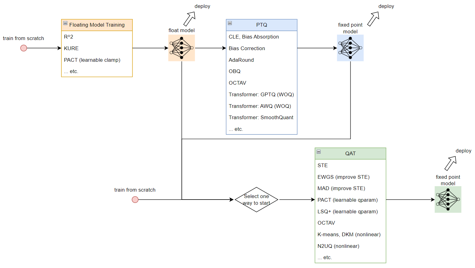
Post Training Quantization (PTQ) 稱事後量化. Quantization Aware Training (QAT) 表示訓練時考慮量化造成的損失來做訓練
為了得到 fixed point model 可以對事先訓練好的 float model 做 PTQ 或 QAT, 或是直接從 QAT 流程開始
同時 QAT 也可以用 PTQ 來初始化訓練. 如果要從 float model 開始做量化的話, 可以考慮在訓練 float model 時就對之後量化能更加友善的技術 (如 R^2, KURE, PACT)

接著對每個技術點盡量以最簡單的方式解說. 如果對量化還不是那麼熟悉, 建議參考一下文章後半段的”簡單回顧量化”

⚠️ 可能寫的比較瑣碎和雜亂, 主要給自己筆記用

令 $f:\mathbb{R}^{n}\rightarrow\mathbb{R}^{m}$ 的 Jacobian matrix 為 $J_f(x)$ 是 $(m\times n)$ 矩陣, 而 Hessian 為 $H_f(x)$ 是 $(m\times n \times n)$ 高維 tensor
 $\circ$ VJP 稱為 Vector-Jacobian Product, $vJ_f(x)$, 其中 $v$ 是 ($1\times m$) 的 row vector
 $\circ$ JVP 稱為 Jacobian-Vector Product, $J_f(x)v$, 其中 $v$ 是 ($n\times 1$) 的 column vector
 $\circ$ HVP 稱為 Hessian-Vector Product, $H_f(x)v$, 其中 $v$ 是 ($n\times 1$) 的 column vector
計算 $vJ_f(x)$ 不用先把矩陣 $J_f(x)$ 求出來再跟 $v$ 相乘, 而是可以直接得到相乘的結果(這樣做還更快), 聽起來有點矛盾對吧~同樣的 JVP 和 HVP 也是如此
本文會說明怎麼高效率計算 VJP, JVP, Jacobian, Hessian, 以及 HVP

主要參考 PyTorch 文章: JACOBIANS, HESSIANS, HVP, VHP, AND MORE: COMPOSING FUNCTION TRANSFORMS

HVP 可以用來有效率地計算 $tr(H_f(x))$, 而這個 term 有時候會被當作 loss 來用, 舉例來說:
 $\circ$ Sliced Score Matching (SSM) 會用到
 $\circ$ EWGS quantization (Network Quantization with Element-wise Gradient Scaling, arxiv) 會用到
 $\circ$ More and details see: Thoughts on Trace Estimation in Deep Learning, 更多例子且有非常深入的討論
總結可以參考文末 Summary
先把 function $f$ 定義好: (名字為predict)

接續上一篇
現在我們可以真正的來探討以下問題了:
 A. 速度的分析: 加速到什麼程度? 跟小模型的速度和準確度有關聯嗎? (想像如果 draft 一直被拒絕, 則小模型都是多跑的)
 B. 運算量的分析: Operation 數 (計算量) 也會減少嗎? 還是會增加?
 C. Memory bandwidth 的分析: 會減少還是增加?
 D. Performance 能維持住嗎 (PPL, WER, BLEU, … 端看 model task 是什麼): 還是會有 degrade?

這是 Transformer inference 的加速, 有人猜測 GPT-4 也使用這個方法: https://archive.ph/2RQ8X
Speculative decoding 做到了不影響準確率情況下直接加速 (不改 model 架構, 不 fine tune, 不做 PTQ 等)
這麼神奇的操作就是利用了一個小模型來先跑一些 tokens, 再由原來的大模型評估或修正.
論文顯示 LLM 效果無損直接可提速 2~3 倍, 讓我們看下去

Motivation

使用 SongHan 教授的課程 slides.
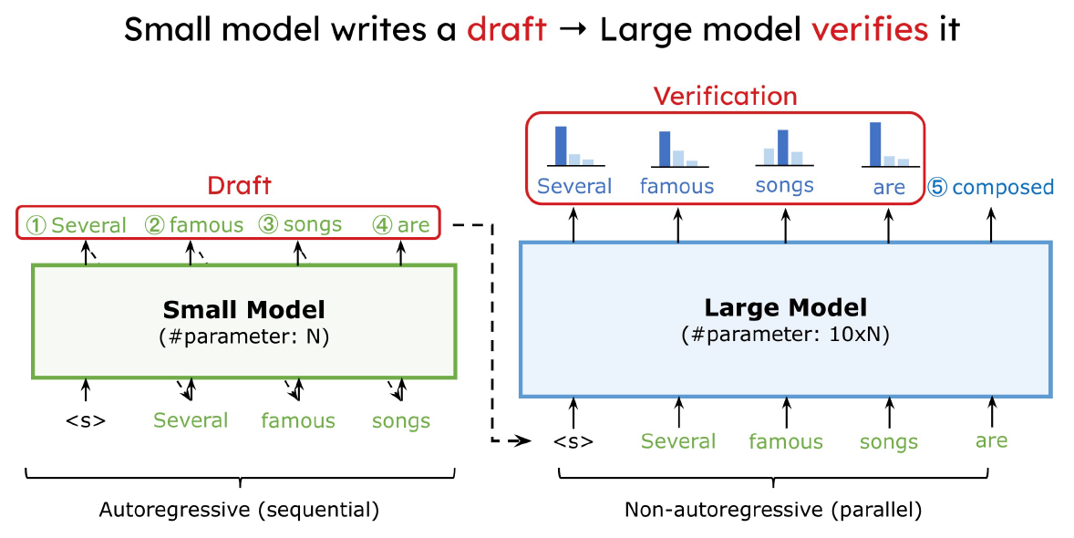利用 small model 先提出一些 draft tokens, 然後用 large model 來驗證. 如果大部分都接受, 直覺上可以省去很多 large model 的呼叫次數, 因此加速. 方法十分簡單, 不過其實魔鬼藏在細節裡, 跟原本只使用 large model 的方法比較有幾個問題要回答:
 A. 速度的分析: 加速到什麼程度? 跟小模型的速度和準確度有關聯嗎? (想像如果 draft 一直被拒絕, 則小模型都是多跑的)
 B. 運算量的分析: Operation 數 (計算量) 也會減少嗎? 還是會增加?
 C. Memory bandwidth 的分析: 會減少還是增加?
 D. Performance 能維持住嗎 (PPL, WER, BLEU, … 端看 model task 是什麼): 還是會有 degrade?
Google 這篇論文很精彩的理論分析了以上所有問題, 並有實務驗證
先破題, performance (PPL, WER, BLEU, …) 可以保證維持住! 我們等到本篇筆記最後在討論, 以下會先討論算法流程、加速和運算量的分析.

如同 SmoothQuant 論文裡的圖, 在 memory size 已經跟不上算力和模型大小情況下, memory bandwidth 已經變成 bottleneck.
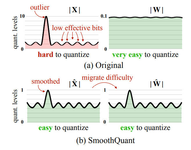
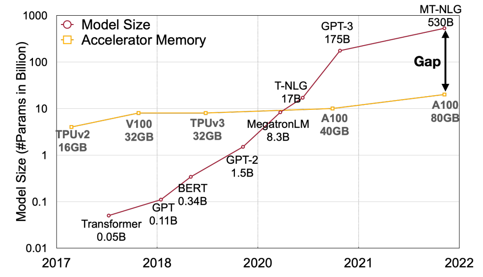如何降低 memory 使用量將變的很關鍵, 因此 Activation-aware Weight Quantization (AWQ) 這篇文章就專注在 Weight Only Quantization (WOQ), 顧名思義就是 weight 使用 integer 4/3 bits, activations 仍維持 FP16.
因為 computation is cheap, memory is expensive.

Intel® Neural Compressor 有實作 WOQ 裡面有 AWQ

以下內容直接筆記 MIT SongHan 教授的課程內容[slides], [Video]

這是 MIT SongHan 教授實驗室的論文, 使用 PTQ 對 LLM 做到 W8A8 的量化, 由於 activations 會有比較大的 outliers 導致 quantization 後損失較大, 而一般 weights 的 outliers 很少, 因此透過一些等價的轉換將 activations 的 scale 縮小並放大 weights 的 scale, 使得 activations 變的較容易 quant 而 weights 仍然容易 quant. 如論文的圖顯示:

總歸來說 Data-Free Quantization (DFQ) 的目的是讓 floating model 做 weights 各種調整, 使得不管是 weights or activations 都變得適合 per tensor 量化.這樣理想上就不需用到 per channel 量化, 因為 per channel 雖然效果很好, 但硬體比較不友善, 且花的運算量較高. 另外 DFQ 屬於 Post-Training Quantization (PTQ) 方法. PTQ 對佈署到 edge 端很方便, 但一般來說 PTQ 都不如 Quantization-Aware Training (QAT) 的效果好, 因此 DFQ 嘗試提升效果.

DFQ 共四步, 對照圖看, 需照順序:

1. Cross-Layer Equalization (CLE): 輸入 fused BN 後的 float model $M_f^1$, floating 操作對 weights 做調整使得更均衡方便 per tensor 量化, 為 step 3 的前置作業, 輸出仍為 float model $M_f^2$.
2. Bias Absorption (BA): 輸入 CLE 後的 float model $M_f^2$, floating 操作對 activations 做調整使得更均衡方便 per tensor 量化, 為 step 3 的前置作業, 輸出仍為 float model $M_f^3$.
3. PTQ 量化: 輸入 CLE+BA 後的 float model $M_f^3$, 此時不管 weights or activations 都適合做 per-tensor 量化了, 所以直接 PTQ 輸出 int model $M_i^1$.
4. Bias Correction (BC): 輸入 float model $M_f^1$ 和 step 3 的 $M_i^1$, 並且(option)給一些 unlabeled 的代表 data, BC 會對 $M_i^1$ 的 bias 參數補償因為量化造成的數值 mean 偏移, 輸出為最終 fixed point model $M_i^2$.

Qualcomm AI Lab 的 tool AIMET 說 BC 這一步驟可以用 AdaRound (需要一小部分的 unlabelled training data) 取代

其實認真看完論文, 覺得限制有點多啊! 很多時候不能套 CLE, 有時 BA 也用不了. 把限制條列一下:

上一篇文章我們提到, uniformly constrained quantizer 有這樣的 quantization error:
$$\begin{align} J=s_{\text max}^2{4^{-B}\over 3} \end{align}$$ 其中 $s_{\text {max}}$ 表示 input $x$ 在 $[-s_{\text {max}}, s_{\text {max}}]$之間.
這麼做雖然能確保所有 $x$ 都不會發生 clipping error, 但如果有一些 outlier 則會使得 quantization step 變很大 (quantization resolution 變低), 因此 quantization 的離散化誤差 (discretization error) 變大.

Quantization error = (Discretization error) + (Clipping error)

舉例來說, 考慮下圖 (ref. from SongHan course EfficientML.ai Lecture 6):

上圖左是 clipping scalar 設定很大, 上圖右則是設定很小. 可以看見 discretization error 跟 clipping error 互為 trade-off.

那麼問題來了, 怎麼設定 clipping scalar, 才會使得整體的 quantization error 最小?
這篇文章 “Optimal Clipping and Magnitude-aware Differentiation for Improved Quantization-aware Training” [arxiv] 給出了理論值, 並使用 Newton’s method 幫助我們很快找到最佳解.

我在閱讀這篇論文: “Optimal Clipping and Magnitude-aware Differentiation for Improved Quantization-aware Training” [arxiv] 的時候, 看到這個式子說明 uniform constrained quantizer 有這樣的 quantization error:
$$\begin{align} J=s_{\text max}^2{4^{-B}\over 3} \end{align}$$ 當下看得我一頭霧水, 後來查了資料才了解這個 quantization error 的推導, 因此筆記一下. [來源1], [來源2]

這裡要特別說明一下, 這邊的 quantization error 沒有考慮超過最大最小值造成的 clipping error. 將 clipping error 一起考慮是開頭說的那篇論文會探討的情況.

這樣的 quantization error 分析在傳統訊號處理可以看到, 例如 analog 訊號經過 ADC 變成 digital 訊號後會有 quantization 損失. 如果 quantization bit 增加 1 bit 則 SNR 增加約 6dB. 又如果採用 nonlinear quantization 則對音量較低的情況其 SNR 提昇會比 linear quantization 好. Nonlinear quantization 又分 $\mu$-law (北美 and 日本) 和 A-law (歐洲 and 其他). 這些內容在下面的筆記都會解釋. Let’s go~

本文是這篇論文 “LoRAPrune: Pruning Meets Low-Rank Parameter-Efficient Fine-Tuning [arxiv]” 的筆記.

一般來說使用 first-order Taylor importance 的 pruning 方法 (下面會介紹此法) 需計算 gradients 來對每個 weight 計算重要性, 然後根據重要性剪枝. 但是現在模型已經愈來愈大, 對所有 weights 都須計算 gradient 的負擔太大.

另一方面, 在 LLM 中對於大模型的 fine tuning 使用 LoRA (PEFT, Parameter Efficient Fine Tuning, 的一種) 來計算 gradients 非常有效率, 原因是對原來的 weights 是 fixed 的, 只 train LoRA 外掛的”少量”參數, 因此只有少量的 gradients 需要計算. 不過我們思考一下, 如果要對已經 prune 的 weights 旁邊外掛 LoRA 的話, LoRA train 完後沒辦法 merge 回去原來的 weights, 因為有可能打亂原本要 prune 的位置. 但是反過來說, 如果先用 LoRA fine tune 完才進行剪枝, 又回到當模型太大而負擔太大沒效率的問題. 況且這樣分兩步驟可能不是很直接, 如果能在 LoRA fine tune 時就能一併考慮某些 weights 會被 prune 的情況下去 fine tune 可能會更好.

如何 pruning 原來的參數又能利用上 LoRA 的效率就是此篇論文的工作.

以下會先介紹 first-order Taylor importance 的 pruning 方法, 再來介紹 LoRA, 最後說明如何取兩者之優點得出此篇的方法: LoRAPrune