import copy

import torch

from common.data import calibration_batches, evaluate, make_loader, train
from common.graph_utils import compare, observer_nodes, qdq_nodes, short, sqnr
from common.models import example_inputs, get_model
from common.pt2e import convert_pt2e, export_module, get_xnnpack_quantizer, prepare_pt2e, quiet
from common.viz import draw, draw_stages, table

quiet()
_ = torch.manual_seed(0)M01-1 | Minimal PTQ: The Four Steps

This notebook takes a small trained model through PT2E post-training quantization (PTQ):
| Step | API | What it does to the graph |
|---|---|---|
| 1. export | torch.export.export |
Turns an nn.Module into an fx graph of ATen ops |
| 2. prepare | prepare_pt2e(graph, quantizer) |
Inserts observers on the edges to quantize, following the quantizer’s annotations |
| 3. calibrate | Call the graph directly | Feed representative data; observers record min/max |
| 4. convert | convert_pt2e(graph) |
Replaces observers with quantize / dequantize nodes |
After each step we draw the same local piece (the very front of the model: conv → bn → relu → max_pool2d) and see how it changes. Just run the cells from top to bottom.
0. First, Train a Usable fp32 Model
TinyConvNet is this project’s small classification network (conv-bn-relu, one residual block, linear), and the data is synthetic 4-class images, so nothing needs to be downloaded. A few epochs of training give over 80% accuracy, so there is something to compare before and after quantization.
model = get_model("tiny")
train_loader = make_loader(2048, seed=0)
test_loader = make_loader(512, seed=7, shuffle=False)
train(model, train_loader, epochs=6, lr=0.05)
model.eval()
acc_fp32 = evaluate(model, test_loader)
print(f"fp32 accuracy = {acc_fp32:.4f}")
fp32 accuracy = 0.88481. export: Turn the Model into a Graph
export_module() calls torch.export.export(model, example_inputs) underneath, and makes the batch dimension dynamic (calibration will feed different batch sizes). The result is a GraphModule: each node is an ATen op.
First list the graph’s operations in order on one line, as a map:
ex = example_inputs()
gm = export_module(model, ex)
print(" → ".join(short(n.target) for n in gm.graph.nodes if n.op == "call_function"))
conv2d → batch_norm → relu → max_pool2d → conv2d → batch_norm → relu → conv2d → batch_norm → add → relu → max_pool2d → conv2d → batch_norm → relu → adaptive_avg_pool2d → flatten → linearFrom here on we draw only this front section. draw()’s focus picks the nodes to look at, and hops=0 means do not expand outward; a dashed “…” means other nodes in the graph attach here but are not drawn. Parameters such as weight and bias are not drawn separately; they are written inside ‹…› under the op that uses them.
STEM = ["conv2d", "batch_norm", "relu", "max_pool2d"]
draw(gm, focus=STEM, hops=0, title="The stem after export")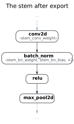
2. prepare: Insert Observers by Annotation
The quantizer decides “which edges get quantized, and with what spec”. It quantizes nothing itself, only puts annotations on node.meta; prepare_pt2e reads these annotations and inserts observers on the corresponding edges. Here we use XNNPACK’s quantizer (is_per_channel=True: one scale per output channel of the weight).
Note that prepare_pt2e modifies the graph you pass in, in place, and returns that same object. We want to keep the exported graph for comparison, so we copy.deepcopy first.
quantizer, src = get_xnnpack_quantizer(is_per_channel=True)
prepared = prepare_pt2e(copy.deepcopy(gm), quantizer)
assert prepared is not gm
print(f"XNNPACKQuantizer source: {src}")
print(f"Number of observers inserted: {len(observer_nodes(prepared))}")
XNNPACKQuantizer source: torchao.testing
Number of observers inserted: 16On the left is the exported graph, on the right the graph after prepare_pt2e. Look for three things:
batch_normis gone: during prepare it is folded into the conv’s weight and bias (M04 covers this in detail).- A
PerChannelMinMaxObserverappears in front of the conv’s weight, andHistogramObserveron the activation edges. - There is no observer between conv and relu: the quantizer treats conv + relu as a group and quantizes only the relu’s output.
draw_stages([(gm, "export"), (prepared, "prepare_pt2e")], focus=STEM, hops=0,
             title="The stem before and after prepare_pt2e(gm, quantizer)")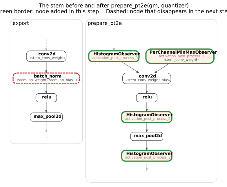
Observers only observe and do not change values, so the graph after prepare produces almost the same output as the original model. The only difference comes from the order of floating-point operations when BN is folded into conv. (We compare on a copy of the graph: if we called prepared directly, the observers would also record this input into the calibration statistics.)
with torch.no_grad():
    s = sqnr(model(*ex), copy.deepcopy(prepared)(*ex))
print(f"Graph after prepare vs fp32 model: SQNR = {s:.1f} dB")
assert not any(short(n.target) == "batch_norm" for n in prepared.graph.nodes)
assert s > 100
Graph after prepare vs fp32 model: SQNR = 126.5 dB3. calibrate: Let the Observers See Data
Feed data directly into the graph after prepare. Each observer records the value range it has seen on its own edge, and later calculate_qparams() converts that into scale and zero point (see this chapter’s overview for the formulas).
with torch.no_grad():
    for batch in calibration_batches(n=256, batch_size=32):
        prepared(*batch)

rows = []
for node, obs in observer_nodes(prepared)[:5]:
    scale, zp = obs.calculate_qparams()
    kind = f"per-channel, {scale.numel()} sets" if scale.numel() > 1 else "per-tensor"
    rows.append([node.name, type(obs).__name__, kind, f"{float(scale.flatten()[0]):.5f}", int(zp.flatten()[0])])
table(rows, ["observer", "type", "granularity", "scale (first set)", "zero point"])| observer | type | granularity | scale (first set) | zero point |
|---|---|---|---|---|
| activation_post_process_1 | PerChannelMinMaxObserver | per-channel, 16 sets | 0.00295 | 0 |
| activation_post_process_4 | PerChannelMinMaxObserver | per-channel, 16 sets | 0.00261 | 0 |
| activation_post_process_6 | PerChannelMinMaxObserver | per-channel, 16 sets | 0.00269 | 0 |
| activation_post_process_10 | PerChannelMinMaxObserver | per-channel, 32 sets | 0.00220 | 0 |
| activation_post_process_14 | PerChannelMinMaxObserver | per-channel, 4 sets | 0.00863 | 0 |
4. convert: observer → quantize / dequantize
convert_pt2e takes the qparams computed by each observer and replaces the observer with a quantize_per_tensor → dequantize_per_tensor pair. The weight side is stored directly as an int8 constant, leaving only a dequantize_per_channel in front of it. convert_pt2e also modifies in place, so again we copy first.
This time hops=1, which also draws the observers adjacent to the stem. In the prepare graph on the left, the observers in dashed boxes disappear after convert; the green-boxed q/dq on the right are the nodes that replace them, and their scale / zp are the same as the ones computed by the observers on the left.
quantized = convert_pt2e(copy.deepcopy(prepared))
draw_stages([(prepared, "prepare_pt2e"), (quantized, "convert_pt2e")], focus=STEM, hops=1,
            title="The stem before and after convert_pt2e(prepared)")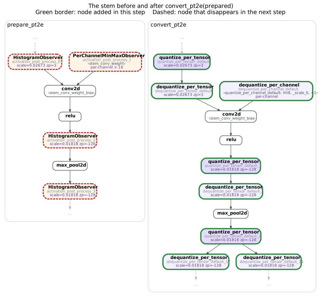
assert not observer_nodes(quantized)
print(f"Number of q/dq nodes: {len(qdq_nodes(quantized))}")
Number of q/dq nodes: 28Acceptance: How Much Accuracy Dropped
SQNR (signal-to-quantization-noise ratio) turns “how far from the fp32 output” into dB; larger means closer.
acc_int8 = evaluate(quantized, test_loader)
stats = compare(model, quantized, ex)
table([
    ["accuracy", f"{acc_fp32:.4f}", f"{acc_int8:.4f}"],
    ["Output SQNR (vs fp32)", "-", f"{stats['sqnr_db']:.1f} dB"],
    ["Max absolute error", "-", f"{stats['max_abs_err']:.4f}"],
], ["", "fp32 model", "Graph after convert"])| fp32 model | Graph after convert | |
|---|---|---|
| accuracy | 0.8848 | 0.8848 |
| Output SQNR (vs fp32) | - | 28.1 dB |
| Max absolute error | - | 0.1204 |
Summary
- Of the four steps, only prepare and convert change the graph; the quantizer only annotates.
- The graph after convert is called a Q/DQ graph: every op is wrapped in q/dq, but conv and relu themselves are still fp32 computations. It simulates int8 numerically and is not faster. Actually switching to int8 kernels is left to the backend (from M07 on).
- The next notebook, M01-2, lays out each change prepare and convert make to the graph.