import copy

import matplotlib.pyplot as plt
import torch
from matplotlib_inline.backend_inline import set_matplotlib_formats

from common.data import calibration_batches, evaluate, evaluate_loss, make_loader, trained_tiny_net
from common.graph_utils import observer_nodes, op_counts, sqnr
from common.models import example_inputs
from common.pt2e import (
    LearnableFakeQuantize,
    MovingAverageMinMaxObserver,
    convert_pt2e,
    enable_range_learning,
    export_module,
    prepare_qat_pt2e,
    quiet,
)
from common.qat import EPS, freeze_for_eval, make_schedule, qat_quantizer, train_qat
from common.viz import table

quiet()
_ = torch.manual_seed(0)
set_matplotlib_formats("svg")
BLUE, ORANGE, MUTED, GRID = "#2a78d6", "#eb6834", "#52514e", "#e6e5e1"M06-5 (Optional) | Range Learning: Make scale/zero_point Trainable Parameters

So far, scale has been decided by the observer’s statistics (a moving average of min/max), and training only changed the weights. LearnableFakeQuantize makes scale and zero_point nn.Parameters, so the loss gradient adjusts the quantization range directly. This is the LSQ approach.
We suggest reading the blog post “Learning Zero-Point and Scale in Quantization Parameters” (in Chinese) first. It explains how LSQ/LSQ+ take gradients with respect to scale and zero_point, and what grad scaling is. Sections B and D are much easier after that.
- A. How to plug it into PT2E: swap the spec to
LearnableFakeQuantize; the parameters are only created after one forward; scale must be clamped back to positive. - B. Gradients: still STE with respect to x; the gradient with respect to scale is nonzero.
- C. The scale trajectory: observer version vs learnable version.
- D. The effect (int4, 3 seeds): observer, learnable, with grad scaling, and with a separate lr for qparams.
The whole notebook takes about 2 minutes to run.
A. Plugging It into PT2E
qat_quantizer(weight_fq="learnable", act_fq="learnable") (common/qat.py) only swaps the spec’s observer_or_fake_quant_ctr for LearnableFakeQuantize.with_args(observer=…); the conv + BN subgraph of prepare_qat_pt2e and convert’s folding work as usual.
Training schedule: for the last 40% (from step 96) BN uses running stats, so that the graph in the last stretch of training is consistent with the convert graph (make_schedule(bn_eval_at=96), a tool in this project’s common/qat.py that calls move_exported_model_to_eval when the given step is reached); in addition, enable_range_learning is called at step 32: first let the observer collect the range for one epoch as the initial value, then start learning. enable_range_learning also turns the observers off, so from then on the range is decided by gradients only.
model = trained_tiny_net()
test_loader = make_loader(n=1024, seed=2, shuffle=False)
(x,) = next(calibration_batches(64, seed=9))
LEARN_AT = 32


def schedule(learn=True):
    bn = make_schedule(bn_eval_at=96)

    def on_step(step, m):
        bn(step, m)
        if learn and step == LEARN_AT:
            m.apply(enable_range_learning)

    return on_step


def prepare(**kw):
    return prepare_qat_pt2e(export_module(copy.deepcopy(model), example_inputs(), train=True), qat_quantizer(bits=4, **kw))


def n_qparams(gm):
    return sum(1 for n, _ in gm.named_parameters() if n.endswith((".scale", ".zero_point")))


prepared = prepare(weight_fq="learnable", act_fq="learnable")
before = n_qparams(prepared)
with torch.no_grad():
    prepared(*example_inputs())
after = n_qparams(prepared)
print("fake quant classes:", {type(m).__name__ for _, m in observer_nodes(prepared)})
print("batch_norm in the graph (QAT subgraph as usual):", op_counts(prepared).get("batch_norm", 0))
print(f"scale/zero_point parameters: {before} before forward, {after} after one forward")
assert before == 0 and after > 0
fake quant classes: {'LearnableFakeQuantize'}
batch_norm in the graph (QAT subgraph as usual): 4
scale/zero_point parameters: 0 before forward, 24 after one forwardscale/zero_point are created lazily: only on the first forward are they initialized into Parameters from the observer’s statistics. The optimizer only remembers the parameters that exist when it is built, so you must forward once before building the optimizer. This is why train_qat forwards once at the start.
The second trap can only be caught with M06-3’s check. By default train_qat clamps scale back to positive after every opt.step() (clamp_scale=True); below we compare turning it off and on:
rows, a = [], {}
for clamp in (False, True):
    p = train_qat(copy.deepcopy(prepared), epochs=5, on_step=schedule(), seed=1, clamp_scale=clamp)
    converted = convert_pt2e(freeze_for_eval(copy.deepcopy(p)))
    bad = [n.name for n, m in observer_nodes(p) if m.scale is not None and float(m.scale.min()) < EPS]
    with torch.no_grad():
        a[clamp] = sqnr(p(x), converted(x))
    rows.append(["yes" if clamp else "no", f"{a[clamp]:.1f}", ", ".join(bad) or "—"])
table(rows, ["Clamp scale back to positive every step", "fake quant graph vs convert graph (dB)", "Fake quants with scale ≤ 0"])| Clamp scale back to positive every step | fake quant graph vs convert graph (dB) | Fake quants with scale ≤ 0 |
|---|---|---|
| no | 2.0 | activation_post_process_4, activation_post_process_10 |
| yes | inf | — |
assert a[False] < 20 and a[True] == float("inf")- Without the clamp, gradients push the scale of some channels negative. Forward still works, because \(\mathrm{round}(w/s)\cdot s\) does not care about the sign of \(s\). Whether it goes negative depends on the training process: with the same settings but BN not switched to eval, none of the 3 seeds tried here went negative, so clamping back to positive at every step is the safe practice.
- torchao 0.18’s
LearnableFakeQuantizeclamps scale to eps only incalculate_qparams(), that is, when convert takes the qparams. The weights of those channels become almost all 0 in the convert graph, and the two graphs are left with single-digit dB at best. - With the clamp back to positive at every step (
clamp_learnable_scales()incommon/qat.py), training and convert use the same scale, and we are back to inf.
B. Gradients: STE with Respect to x, Nonzero with Respect to scale
A single int4 LearnableFakeQuantize, with the range initialized on [-1, 1] and then range learning turned on:
fq = LearnableFakeQuantize(observer=MovingAverageMinMaxObserver, quant_min=-8, quant_max=7, dtype=torch.int8,
                           qscheme=torch.per_tensor_affine, eps=EPS)
with torch.no_grad():
    fq(torch.linspace(-1, 1, 100))
fq.enable_range_learning()
xs = torch.tensor([-3.0, -0.5, 0.0, 0.3, 0.9, 1.5, 4.0], requires_grad=True)
fq(xs).sum().backward()
assert xs.grad is not None and fq.scale is not None and fq.scale.grad is not None
table([["dfq/dx", *(f"{float(g):.0f}" for g in xs.grad)]], ["x", *(f"{float(v):+.1f}" for v in xs)])| x | -3.0 | -0.5 | +0.0 | +0.3 | +0.9 | +1.5 | +4.0 |
|---|---|---|---|---|---|---|---|
| dfq/dx | 0 | 1 | 1 | 1 | 1 | 0 | 0 |
print(f"scale = {float(fq.scale):.4f}, d(sum fq)/d(scale) = {float(fq.scale.grad):.3f}")
assert float(fq.scale.grad) != 0
scale = 0.1333, d(sum fq)/d(scale) = 5.750The gradient with respect to x is STE, the same as in M06-1. The gradient with respect to scale (LSQ): inside the range it is \(\mathrm{round}(x/s) - x/s\), and outside the range it is \(q_{min}\) or \(q_{max}\). Clamped values push scale larger, and the round error inside the range pushes scale smaller; which way it goes is decided by the loss, no longer by min/max. use_grad_scaling=True divides the gradient of scale by \(\sqrt{\text{numel} \times q_{max}}\) (the LSQ paper’s suggestion); section D looks at its effect.
C. The scale Trajectory
Record the scale of the input’s fake quant (activation_post_process_0), once every 32 steps:
traj = {}
for name, kw, learn in (("observer", {}, False), ("learnable", dict(weight_fq="learnable", act_fq="learnable"), True)):
    t = []

    def log(step, m, t=t):
        if step % 32 == 0:
            t.append(float(m.get_submodule("activation_post_process_0").calculate_qparams()[0]))

    train_qat(prepare(**kw), epochs=5, on_step=schedule(learn), seed=1, log=log)
    traj[name] = t
STEPS = list(range(32, 161, 32))
Plotting code
fig, ax = plt.subplots(figsize=(6.4, 3.0))
for (name, t), color in zip(traj.items(), (MUTED, BLUE)):
    ax.plot(STEPS, t, color=color, lw=2, marker="o", ms=5)
    ax.annotate(name, (STEPS[-1], t[-1]), xytext=(6, 0), textcoords="offset points", va="center", color=color, fontsize=9)
ax.axvline(LEARN_AT, color=MUTED, lw=0.8, ls="--")
ax.annotate("range learning on", (LEARN_AT, min(min(t) for t in traj.values())), xytext=(4, 0),
            textcoords="offset points", color=MUTED, fontsize=8, va="bottom")
ax.set_xlim(20, 190)
ax.set_xlabel("training step", color=MUTED)
ax.set_ylabel("input scale", color=MUTED)
ax.grid(axis="y", color=GRID, lw=0.8)
ax.spines[["top", "right"]].set_visible(False)
ax.tick_params(colors=MUTED)
plt.show()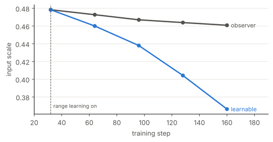
assert traj["learnable"][-1] < traj["observer"][-1]The observer version’s scale only drifts slowly with the moving average; the learnable version is continuously pushed smaller by gradients from step 32 on: it shrinks the range to get a finer grid inside the range, at the cost of clamping more values.
D. The Effect
int4, lr 1e-3, BN eval @96, 3 seeds per setting. Evaluation uses the fake quant graph after freeze (section A already confirmed it equals the convert graph):
CONFIGS = {
    "observer (range not learned)": ({}, {}),
    "learnable": (dict(weight_fq="learnable", act_fq="learnable"), {}),
    "learnable + grad scaling": (dict(weight_fq="learnable", act_fq="learnable", grad_scaling=True), {}),
    "learnable + grad scaling, qparams lr 1e-2": (dict(weight_fq="learnable", act_fq="learnable", grad_scaling=True),
                                                 dict(qparams_lr=1e-2)),
    "learnable, qparams lr 1e-2 (no grad scaling)": (dict(weight_fq="learnable", act_fq="learnable"), dict(qparams_lr=1e-2)),
}
d = {}
for name, (qkw, tkw) in CONFIGS.items():
    base, losses, accs = prepare(**qkw), [], []
    for seed in (1, 2, 3):
        p = freeze_for_eval(train_qat(copy.deepcopy(base), epochs=5, on_step=schedule(name != "observer (range not learned)"),
                                      seed=seed, **tkw))
        losses.append(evaluate_loss(p, test_loader))
        accs.append(evaluate(p, test_loader))
    d[name] = (losses, sum(accs) / 3)
table([[name, f"{sum(v) / 3:.3f}", f"{min(v):.3f} ~ {max(v):.3f}", f"{acc:.3f}"] for name, (v, acc) in d.items()],
["Setting", "Mean test loss", "min ~ max", "Mean accuracy"])| Setting | Mean test loss | min ~ max | Mean accuracy |
|---|---|---|---|
| observer (range not learned) | 0.831 | 0.729 ~ 1.027 | 0.733 |
| learnable | 0.779 | 0.704 ~ 0.818 | 0.694 |
| learnable + grad scaling | 0.783 | 0.693 ~ 0.881 | 0.731 |
| learnable + grad scaling, qparams lr 1e-2 | 0.867 | 0.752 ~ 1.037 | 0.704 |
| learnable, qparams lr 1e-2 (no grad scaling) | 1.399 | 1.386 ~ 1.411 | 0.252 |
obs, learn = d["observer (range not learned)"][0], d["learnable"][0]
gs = d["learnable + grad scaling"][0]
# Which of the first four settings is best depends on the platform and the seeds (see the notes below); only divergence is stable.
assert d["learnable, qparams lr 1e-2 (no grad scaling)"][1] < 0.3 # diverges: accuracy near random guessing over 4 classes- Switch to learnable (nothing else changed): the mean test loss is lower than the observer version on both platforms (macOS arm64: 0.757 vs 0.883; Linux x86, shown here: 0.779 vs 0.831), and the range across seeds is the narrowest or close to it. On macOS arm64 all 3 seeds beat the observer version; on Linux x86 the ranges overlap (learnable 0.704 ~ 0.818, observer 0.729 ~ 1.027), so “wins on every seed” does not hold there. The training is not bit-reproducible across platforms even from the same starting weights, which is why only the mean is a fair comparison.
- Add grad scaling: the gradient of scale becomes smaller and it moves slowly. On macOS arm64 this made the mean worse than plain learnable and the range wider (0.840, 0.753 ~ 0.941); on Linux x86 it is about the same as plain learnable (0.783) with a wider range. Raising the lr of qparams on top of it did not help on either platform (0.806 on macOS, 0.867 on Linux).
- No grad scaling but qparams lr 1e-2: it diverges outright, and accuracy drops to random guessing over 4 classes (on both platforms). The lr of scale and grad scaling are tied together and can only be tuned together.
- This is the result of a single model and 3 seeds. The settings that differ by about 0.05 in mean loss swap places between the two platforms, so differences of that size are within the noise; whether “better without grad scaling” (or the opposite) holds on other models is not verified here.
Summary
- Plugging it into PT2E only needs a spec swap; but the optimizer must be built after one forward, and scale must be clamped back to positive at every step, otherwise training graph ≠ convert graph.
- Range learning also hands the range to the loss to decide; the cost is an extra set of hyperparameters (grad scaling, the lr of qparams), and a wrong choice diverges. On this small model it beat the observer version on the mean on both platforms, but not on every seed on every platform.